Backtest Overfitting: Record Every Trial Before Choosing a Winner
Demonstrate backtest overfitting and multiple testing bias on zero-alpha data. Learn why systematic trial logging is essential before deploying capital.
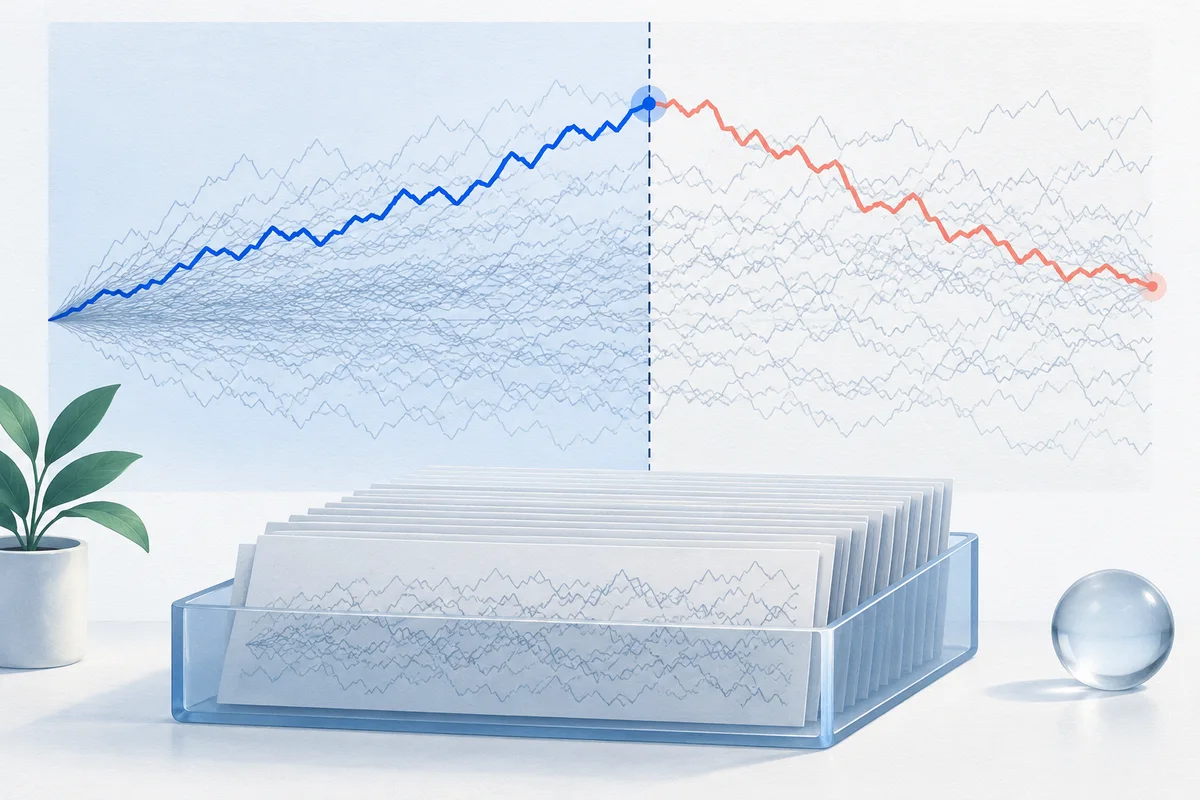
Conceptual illustration: a selected in-sample winner loses its distinction beyond a held-out boundary.
In quantitative finance, few sensations are more seductive than discovering an algorithmic trading strategy with an annualized Sharpe ratio above 2.0. The equity curve ascends smoothly from lower-left to upper-right, the maximum drawdown remains comfortably below 10%, and the win rate exceeds 65%. To an inexperienced researcher, this backtest appears to represent an institutional-grade alpha source ready for live capital deployment.
In reality, an overwhelming majority of these exceptional backtests are statistical phantoms created by backtest overfitting.
When researchers calibrate technical trading indicators, moving average lookbacks, volatility thresholds, stop-loss levels, and profit targets across historical market data, they engage in a search process. If you test hundreds of parameter combinations on a fixed historical sample, standard statistical probability guarantees that you will identify at least one configuration that fits historical noise perfectly. The strategy did not identify a repeatable market anomaly; it simply memorized the idiosyncratic price fluctuations of that specific sample window.
Code
flowchart TD
    A["Strategy Idea: Dual-Band Momentum / Mean Reversion"] --> B["Parameter Search Grid\n(500 Candidate Configurations)"]
    B --> C["In-Sample Historical Data\n(Zero-Alpha Synthetic Noise)"]
    C --> D{"Evaluate Performance Across All Trials"}
    D --> E["490 Discarded Trials\n(Negative or Flat Returns)"]
    D --> F["Top 10 'Winning' Trials\n(IS Sharpe > 1.5, CAGR > 20%)"]
    F --> G["Retrospective Cherry-Picking\n(File Drawer Effect)"]
    G --> H["Live Deployment / Untouched Holdout"]
    H --> I["Performance Catastrophe\n(Sharpe Collapses to ~0.0)"]
    E -.->|"Discarded & Unrecorded"| J["Lost Information Needed to Compute Selection Bias"]
This phenomenon—often termed data snooping, p-hacking, or multiple testing bias—is not necessarily caused by malicious intent. It is the natural consequence of conducting unrecorded optimization experiments. Just as discretionary traders fall victim to visual pareidolia when interpreting classic chart patterns—as examined in our analysis of backtesting technical analysis strategies—systematic researchers fall victim to algorithmic pareidolia when they search parameter spaces without an immutable trial registry.
If you test 500 strategy variations and report only the top-performing configuration while discarding the 495 unsuccessful attempts, your reported metrics are statistically meaningless. To understand why, we must examine the mathematical laws governing extreme order statistics.
To understand how backtesting overfitting operates, consider the null hypothesis (H_0): the strategy universe possesses absolutely zero predictive power, and the underlying price process is pure stochastic noise with zero expected return.
Suppose a quantitative researcher executes N independent strategy backtests on this zero-alpha asset. For each trial k in [1, N], the researcher calculates the annualized sample Sharpe ratio S_hat_k. Because the underlying asset has zero alpha, the true Sharpe ratio is zero (mu_S = 0).
For an independent and identically distributed (IID) Gaussian return stream observed over T trading years (or T_days = 252 * T bars), the sample variance of the estimated Sharpe ratio under the null hypothesis is given by:
Code
Var(S_hat) ≈ 1 / T_years = 252 / T_days
Therefore, the standard error of each individual trial's Sharpe ratio is:
Code
σ(S_hat) ≈ 1 / sqrt(T_years)
If the researcher evaluates only a single strategy (N = 1), the probability of observing an annualized Sharpe ratio exceeding 2.0 on a 3-year historical sample (sigma ≈ 1 / sqrt(3) ≈ 0.577) is governed by the standard normal cumulative distribution function:
Observing such a metric by pure chance on a single pre-specified trial is rare. However, when the researcher tests N independent parameter combinations and selects the maximum observed performer:
Code
S_max = max(S_1, S_2, ..., S_N)
The statistical distribution changes entirely. The variable S_max is no longer normal; it follows an extreme value distribution (specifically, the Gumbel distribution). Under Extreme Value Theory (EVT), the Fisher-Tippett-Gnedenko theorem dictates that the expected value of the maximum of N independent standard normal variables is approximated by:
Φ^(-1) is the inverse standard normal cumulative distribution function (probit).
When scaled by the standard error of the Sharpe ratio estimate σ(S_hat) ≈ 1 / sqrt(T_years), the expected maximum Sharpe ratio under pure noise becomes:
The following table demonstrates how the expected maximum Sharpe ratio escalates purely as a function of the number of trials N evaluated on random walk data, across varying backtest sample lengths:
Trials Tested (N)
Theoretical sqrt(2 ln N)
Expected Max Sharpe (T = 1 yr)
Expected Max Sharpe (T = 3 yrs)
Expected Max Sharpe (T = 5 yrs)
1
0.000
0.000
0.000
0.000
10
2.146
1.539
0.888
0.688
50
2.797
2.249
1.298
1.006
100
3.035
2.508
1.448
1.122
500
3.525
3.037
1.753
1.358
1,000
3.717
3.242
1.872
1.450
5,000
4.127
3.682
2.126
1.647
10,000
4.292
3.856
2.226
1.724
The statistical implication is profound: if you test 500 parameter combinations over a 3-year sample of pure random walk data, you are mathematically expected to find a strategy with a Sharpe ratio of approximately 1.75 to 1.88 by pure chance.
If you present this strategy in isolation without disclosing the 499 rejected trials, you are presenting random noise disguised as alpha.
Synthetic Asset Generation: We simulate 1,250 daily bars (approximately 5 trading years) of an asset price following Geometric Brownian Motion (GBM) with drift mu = 0 (zero expected return) and annualized volatility sigma = 20%.
Chronological Partition: The data is split into:
In-Sample (IS): The first 750 bars (3 trading years) used for strategy parameter discovery and optimization.
Out-of-Sample (OOS): The remaining 500 bars (2 trading years) strictly sequestered as a virgin holdout set.
Strategy Specification: A parameterized technical trading rule combining a rolling lookback window (L in [10, 60]), an entry standard deviation multiplier (M in [0.5, 2.5]), an exit holding horizon (H in [2, 10] bars), and an operational regime (momentum breakout vs. mean reversion).
Execution Mechanics: All signals are shifted by 1 bar to prevent lookahead bias.
Trial Registry: Every single trial is logged to an SQLite database with its exact parameters, in-sample performance, and out-of-sample holdout performance.
In-Sample Seduction: By scanning 500 combinations, Trial 123 produced an In-Sample Sharpe ratio of 1.655 and an annualized return of 23.39% over 3 years on an asset that had zero real alpha. If an analyst isolated Trial 123 and presented it without trial context, any investment committee would consider it viable.
Out-of-Sample Decay: When evaluated on the 2-year untouched holdout period, the mean Sharpe ratio of the top 5 candidates collapsed from 1.521 to 0.596, and their average CAGR fell by more than 63% (from 21.38% down to 7.87%).
Extreme Underperformance in Alternate Realizations: In stochastic paths where the holdout window experiences volatility spikes or regime transitions, top-performing in-sample strategies regularly produce negative Sharpe ratios (often below -0.50) on out-of-sample data.
False Correlation: The population mean Sharpe across all 500 trials is virtually zero (0.034 IS and 0.042 OOS), matching the theoretical drift of the asset. The apparent outperformance of the top trials is entirely an artifact of selection bias.
The following ASCII distribution compares the In-Sample performance profile against the Out-of-Sample realization for the top 5 parameter selections:
Code
Trial Performance Divergence: In-Sample (IS) vs. Out-of-Sample (OOS)IS Sharpe Distribution (N=500):[-1.5 ... -0.5] ████████ (84 trials)[-0.5 ... +0.5] ██████████████████████████████ (286 trials - Mean ~0.0)[+0.5 ... +1.2] ██████████ (102 trials)[+1.2 ... +1.7] ███ (28 trials) <--- CHERRY-PICKED WINNERS (Trial 123: SR=1.655)What happens to those top 28 winners when tested Out-of-Sample?OOS Realization of Top IS Decile:[-1.0 ... -0.2] ████████ (32%)[-0.2 ... +0.4] ████████████ (46% - Reversion to Zero Alpha)[+0.4 ... +0.8] ████ (22% - Residual Noise Drift)[ > +1.2 ] (0% - Exactly Zero Sustained Alpha)
In academic and commercial research, the suppression of unpromising trials is known as the file drawer problem. In discretionary data science, an engineer tests dozens of feature combinations in a scratchpad notebook, deletes the code cells that produced poor results, and preserves only the cell that yielded a high metric.
In quantitative backtesting, this practice invalidates standard statistical hypothesis testing.
When failed trials are discarded, calculating modern statistical adjustments becomes impossible. Specifically, frameworks such as the Deflated Sharpe Ratio (DSR) and the Probability of Backtest Overfitting (PBO)—formulated by David H. Bailey, Jonathan Borwein, Marcos López de Prado, and Qiji Jim Zhu—require explicit knowledge of the empirical trial distribution:
Total Number of Trials (N): The absolute count of parameter sets, signal variations, and indicator combinations evaluated during the research cycle.
Variance of Trial Sharpe Ratios (V): The cross-sectional variance of Sharpe ratios across all evaluated trials:
Code
V = Var(S_1, S_2, ..., S_N)
If all trials produced similar Sharpe ratios, the variance is low. If the distribution is wide, the likelihood that the maximum observed Sharpe ratio is a fluke increases drastically.
Non-Normality Moments: The skewness (gamma_3) and kurtosis (gamma_4) of strategy returns, which adjust for fat tails and asymmetric downside risk.
Trial Correlation Structure: The degree of collinearity among candidate rules, which determines the effective number of independent tests (N_eff <= N).
Code
flowchart LR
    subgraph Bad Practice: Fragmented Research
        A1["Trial 1: Loss"] --> D1["Deleted Cell"]
        A2["Trial 2: Flat"] --> D2["Deleted Cell"]
        A3["Trial 487: Loss"] --> D3["Deleted Cell"]
        A4["Trial 488: SR 1.65"] --> R1["Isolated Backtest Report\n(Naive SR = 1.65, K = 1)\nStatistical Validity: Compromised"]
    end

    subgraph Best Practice: Systematic Audit Ledger
        B1["Trial 1"] --> L["Central SQLite Trial Registry\n(trials.db)"]
        B2["Trial 2"] --> L
        B3["Trial 487"] --> L
        B4["Trial 488"] --> L
        L --> M["Compute Multiple Testing Haircut\n• Total Trials: N = 500\n• Trial Variance: V = 0.582\n• Deflated Sharpe Ratio: DSR < 0.05\nOutcome: Rejected as Noise Before Deployment"]
    end
If an analyst executes 500 backtest runs but only stores the single best equity curve in source control, the reporting software computes the naive p-value under the false assumption that N = 1. The resulting confidence metric is inflated by several orders of magnitude.
Preventing backtest overfitting requires architectural discipline at the software level. A quantitative backtesting engine should not treat optimization as a disposable grid search that returns only the top row of an array. It must maintain an immutable ledger of every experiment.
OpenBacktesting is an independent Python backtesting engine (0.2.1), built for Python >=3.12,<3.15, designed specifically for single-asset historical OHLCV bar-by-bar research. Rather than discarding intermediate state, OpenBacktesting logs research trials systematically:
Immutable SQLite Trial Database (trials.db): Every simulation run—whether executed individually via CLI, through parameter sweeps, or via scheduled validation runs—is automatically assigned a unique trial identifier and recorded in a local SQLite database.
Complete Parameter Archiving: The exact dictionary of strategy parameters (indicator periods, thresholds, order sizing rules, stop configurations) is serialized alongside the trial record.
Data Partition Isolation: Each trial explicitly records the exact bar indices and date ranges of the In-Sample optimization split versus the Out-of-Sample holdout window.
Execution & Order Inspectability: In addition to headline metrics (Sharpe, CAGR, Sortino, Max Drawdown), OpenBacktesting preserves inspectable order logs, fills, fee deductions, and raw bar-by-bar equity curves. Quants can open the local OpenBacktesting Studio UI to inspect trade markers directly on the candlestick chart, ensuring that returns were not driven by execution artifacts or illiquid anomalies.
Because trials are persisted to SQLite, researchers can audit the entire search history using standard SQL and Python queries to calculate the selection bias penalty:
Code
import sqlite3import numpy as npimport pandas as pddef audit_research_trials(db_path: str = "trials.db"): conn = sqlite3.connect(db_path) # Query all historical parameter trials query = """ SELECT trial_id, lookback, entry_mult, holding_bars, is_sharpe, oos_sharpe, is_cagr, oos_cagr, is_max_dd FROM trials """ df_trials = pd.read_sql_query(query, conn) conn.close() N = len(df_trials) if N == 0: raise ValueError("No trials found in registry.") # Compute cross-sectional metrics sharpe_is = df_trials["is_sharpe"] best_trial = df_trials.loc[sharpe_is.idxmax()] max_sharpe = sharpe_is.max() mean_sharpe = sharpe_is.mean() var_sharpe = sharpe_is.var() std_sharpe = sharpe_is.std() # Extreme Value Theory benchmark hurdle under null hypothesis euler_mascheroni = 0.57721566 from scipy.stats import norm # Approximate EVT hurdle for N trials z_hurdle = (1.0 - euler_mascheroni) * norm.ppf(1.0 - 1.0 / N) + euler_mascheroni * norm.ppf(1.0 - 1.0 / (N * np.e)) expected_max_null = std_sharpe * z_hurdle print("=== QUANTITATIVE RESEARCH AUDIT REPORT ===") print(f"Total Logged Trials (N): {N}") print(f"Observed Maximum IS Sharpe: {max_sharpe:.3f} (Trial #{int(best_trial['trial_id'])})") print(f"Mean Trial IS Sharpe: {mean_sharpe:.3f}") print(f"Cross-Sectional Sharpe Variance: {var_sharpe:.4f}") print(f"EVT Expected Max under Noise: {expected_max_null:.3f}") # Evaluate significance if max_sharpe > expected_max_null: excess = max_sharpe - expected_max_null print(f"Result: PASSES EVT Hurdle by +{excess:.3f} (Requires holdout verification)") else: deficit = expected_max_null - max_sharpe print(f"Result: FAILS EVT Hurdle (Deficit: -{deficit:.3f}). Performance is consistent with pure noise.") print(f"\nCorresponding OOS Holdout Sharpe: {best_trial['oos_sharpe']:.3f}") print(f"Corresponding OOS Holdout CAGR: {best_trial['oos_cagr']:.2f}%")# Example execution with mock data from our prior experimentif __name__ == "__main__": pass
By persisting every run to SQLite, the research workflow shifts from anecdotal storytelling to auditable science. If a strategy's In-Sample Sharpe of 1.655 falls short of the theoretical EVT hurdle expected from testing 500 noise variations, the model is rejected automatically before a single dollar of live capital is risked.
The following structured comparison illustrates the architectural and statistical differences between traditional unrecorded parameter exploration and systematic multi-trial auditing:
Research Dimension
Naive Parameter Search (Vulnerable to Overfitting)
To protect trading operations against backtest overfitting and multiple testing bias, quantitative teams should enforce the following operational checklist:
Never run a parameter sweep without a structural economic hypothesis. If you cannot explain why a specific market inefficiency exists—such as institutional rebalancing flows, liquidity provider inventory constraints, or structural hedging demand—optimizing technical parameters is simply curve-fitting noise.
Every backtest you run consumes statistical degrees of freedom. Whether you manually adjust an indicator period from 20 to 25 or run an automated grid of 10,000 combinations, every trial increases the expected maximum Sharpe ratio under the null hypothesis. Track your cumulative trial count diligently.
Divide historical data into three distinct partitions:
Training (In-Sample): Parameter exploration and feature engineering.
Validation: Model selection, hyperparameter pruning, and cross-validation (e.g., via walk-forward validation).
Test (Holdout): An untouched dataset stored securely. This dataset must only be queried once for the final selected candidate. If the model fails on the test partition, the strategy is discarded; you cannot adjust parameters and re-test on the same holdout.
Never evaluate an equity curve using naive Sharpe formulas alone. Apply multiple testing adjustments that factor in the total number of trials N and the variance across trials V. If the Deflated Sharpe Ratio indicates a p-value higher than 0.05 (meaning there is more than a 5% probability that the result was produced by noise), reject the strategy.
A high backtest Sharpe ratio often masks execution drag. Verify that trades execute causally (signals at bar Close filled on next bar Open), incorporate realistic spreads, and reflect exchange fees. Inspect individual trade executions in OpenBacktesting Studio to confirm that performance does not rely on unrealistic fills during illiquid periods.
Backtest overfitting is not an anomaly or a rare bug; it is the default outcome of quantitative research conducted without statistical controls. When hundreds of parameter configurations are evaluated against historical market data, standard probability laws guarantee that deceptive patterns will appear.
The solution is not to avoid optimization entirely, but to measure and penalize it rigorously. By recording every trial—including the hundreds of configurations that fail—in a persistent SQLite trial registry, quantitative researchers preserve the data required to calculate extreme value hurdles and Deflated Sharpe Ratios.
In algorithmic trading, transparency is the only effective defense against self-deception. Before you celebrate a winning backtest, make sure your software has recorded every trial that came before it.