Moving beyond console prints: Why visualization matters in strategy research
Quantitative strategy development often begins in a terminal. A developer writes a Python script, runs a historical simulation, and evaluates a wall of text summarizing the outcome:
======================= BACKTEST SUMMARY =======================
Initial Capital:         $10,000.00
Ending Capital:          $24,250.80
Total Return:            +142.51%
CAGR:                    +10.42%
Sharpe Ratio:            1.84
Sortino Ratio:           2.31
Max Drawdown:            -14.12%
Total Closed Trades:     148
Win Rate:                54.05%
Profit Factor:           1.92
================================================================
On paper, this strategy appears robust. A Sharpe ratio of 1.84 and a maximum drawdown of 14.12% suggest an investable edge. However, relying strictly on scalar metrics hides critical structural risks:
- Drawdown duration and regime blindness: A maximum drawdown of -14.12% sounds manageable, but scalar outputs do not reveal whether that drawdown resolved in three days or endured across an agonizing eighteen-month stagnation regime. If a strategy remains underwater for hundreds of bars, an operator in live trading will likely abandon it long before it recovers.
- Outlier profit dependency: A 142.51% total return can easily be generated by two anomalous earnings gaps rather than consistent statistical edge. If you remove the top three winning trades and the cumulative return collapses to negative, the strategy is an artifact of lucky timing rather than repeatable alpha.
- Execution causality and fill timing: Console prints summarize completed trades without showing when orders were staged, matched, or filled. You cannot verify whether your entry filled at the current bar's close (an unachievable lookahead print) or executed on the next bar's open.
- Clustered execution friction: Console summaries aggregate total commission and slippage costs into a single dollar figure. They fail to highlight whether transaction friction systematically decimated returns during low-volatility chop regimes.
[!IMPORTANT] A backtesting dashboard is not cosmetic eye-candy; it is a verification firewall. Reconciling equity trajectories against drawdown phases, candlestick charts, and granular order fills separates genuine market edge from statistical noise.
Introducing OpenBacktesting Studio: Local, private, and interactive
Modern quantitative developers are often forced to choose between two extremes: bare-bones Python scripts with static chart popups, or cloud-based software-as-a-service (SaaS) platforms that require uploading sensitive IP and proprietary data to remote servers.
OpenBacktesting Studio bridges this gap. It provides a local, browser-based graphical interface that runs directly against your local Python files and datasets.
┌────────────────────────────────────────────────────────────────────────┐
│                        LOCAL WORKSTATION (macOS)                       │
│                                                                        │
│  ┌───────────────────────┐             ┌────────────────────────────┐  │
│  │   Python Strategies   │             │   Local Datasets           │  │
│  │   (.py script files)  │             │   (Parquet / CSV / DataFrames)│
│  └───────────┬───────────┘             └─────────────┬──────────────┘  │
│              │                                       │                 │
│              ▼                                       ▼                 │
│  ┌──────────────────────────────────────────────────────────────────┐  │
│  │             OpenBacktesting Engine (Python >=3.12, <3.15)        │  │
│  │             - Bar-by-bar deterministic simulation                │  │
│  │             - Realistic order matching & friction models         │  │
│  │             - Local SQLite trial persistence                     │  │
│  └──────────────────────────────────┬───────────────────────────────┘  │
│                                     │                                  │
│                                     ▼ IPC / Local Loopback             │
│  ┌──────────────────────────────────────────────────────────────────┐  │
│  │                    OpenBacktesting Studio                        │  │
│  │          (Local Browser Dashboard · Zero Cloud Telemetry)        │  │
│  │  - Strategy Editor & Runner       - Equity & Underwater Curves   │  │
│  │  - Ticket-Level Trade Ledger      - Multi-Parameter Heatmaps     │  │
│  │  - Candlestick Fill Visualizer    - Immutable JSON Exporter      │  │
│  └──────────────────────────────────────────────────────────────────┘  │
└────────────────────────────────────────────────────────────────────────┘
Studio is designed around three architectural commitments:
- Local data privacy: Your strategy source code, trading logic, alpha factors, and proprietary market data never leave your computer. There are no remote uploads, external analytics beacons, or third-party cloud dependencies.
- No remote code execution risks: Strategy simulation executes within your local Python virtual environment. You maintain full access to scientific libraries (
numpy,pandas,pandas-ta-classic,scipy) without running inside restrictive cloud containers. - Offline-first operation: The entire application functions without an internet connection. You can conduct quantitative research in disconnected lab environments, air-gapped workstations, or while traveling.
Key dashboard components in OpenBacktesting Studio
OpenBacktesting Studio organizes the quantitative validation workflow into five specialized modules, enabling researchers to transition from code to granular auditability in a single workspace.
1. The Strategy Editor & Runner
Studio features an embedded code workspace that connects directly to your filesystem. You can edit Python strategy files in the dashboard or use an external IDE such as VS Code, Neovim, or PyCharm with automatic disk synchronization.
The runner interface allows researchers to configure simulation inputs before triggering a backtest:
- Capital & Sizing: Set initial cash and position sizing thresholds (e.g., fixed units or fractional portfolio capital).
- Execution Settings: Specify execution timing (
next_openvs. limit matching), order types, and end-of-test liquidation policies (close_at_last_close). - Transaction Friction: Configure exact broker commissions (percentage or fixed per share) and slippage models (basis points or ATR-based spread impact).
- Live Execution Logging: Monitor bar-by-bar progress and view framework logs in real time, catching unhandled indicator
NaNvalues or margin rejections immediately.
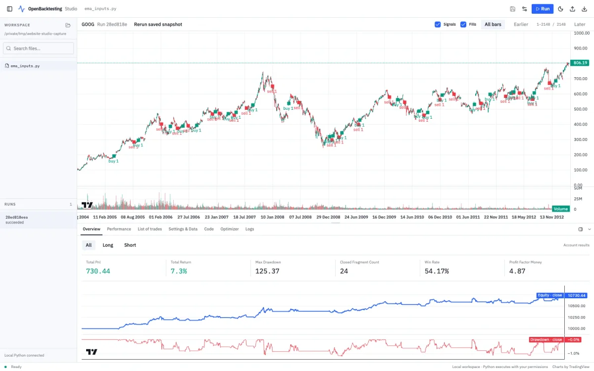
2. The Performance Overview
Once a backtest completes, Studio renders an interactive performance dashboard consisting of two synchronized time-series panels and a risk scorecard:
┌────────────────────────────────────────────────────────────────────────┐
│ Equity Curve                                             [USD] $24,250 │
│  $25k ──┐                                                    ╭──────── │
│  $20k ──┼───────────────────────────────────────╭────────────╯         │
│  $15k ──┼──────────────────────╭────────────────╯                      │
│  $10k ──┴─── Buy & Hold* ──────┴────────────────────────────────────── │
│         2005        2007             2009             2011        2013 │
├────────────────────────────────────────────────────────────────────────┤
│ Underwater Drawdown                                      [% Peak] -14% │
│    0% ──┬───┬───┬───┬───────────────────────────────────┬───┬───────── │
│   -5% ──│   │   ╰───╯                                   │   │          │
│  -10% ──│   ╰─────────────────────────╮                 ╰───╯          │
│  -15% ──┴─────────────────────────────┴─────────────────────────────── │
│         2005        2007             2009             2011        2013 │
└────────────────────────────────────────────────────────────────────────┘- Strategy Equity vs. Benchmark: Plots the strategy equity curve alongside a normalized buy-and-hold price reference, allowing immediate visual attribution of outperformance or underperformance across market cycles.
- Underwater Drawdown Profile: Maps percentage declines below prior equity highs. This panel highlights drawdown severity, duration, and plateau phases, helping researchers identify structural regime vulnerability.
- Standardized Performance Metrics: Displays risk-adjusted ratios, including Sharpe, Sortino, and Calmar ratios, alongside win rates, profit factors, and total trade counts.
3. The Trade & Order Inspector
Evaluating high-level return metrics without reviewing the underlying trade ledger invites severe survivorship and execution bias. The Trade & Order Inspector provides a complete, ticket-level audit table of every simulated execution:
| Ticket ID | Side | Entry Time | Exit Time | Entry Price | Exit Price | Size | Return | Net P&L | Exit Reason |
|---|---|---|---|---|---|---|---|---|---|
#001 | LONG | 2005-01-14 | 2005-03-08 | `98.40 | `104.20 | 95 | +5.89% | +$551.00 | Signal Exit |
#002 | LONG | 2005-04-12 | 2005-05-02 | `96.10 | `91.50 | 102 | -4.79% | -$469.20 | Stop Loss |
#003 | SHORT | 2005-06-20 | 2005-07-15 | `112.30 | `108.10 | 90 | +3.74% | +$378.00 | Take Profit |
#004 | LONG | 2005-08-01 | 2005-08-25 | `105.80 | `114.70 | 92 | +8.41% | +$818.80 | Signal Exit |
#005 | LONG | 2005-09-19 | 2005-10-14 | `120.50 | `116.80 | 85 | -3.07% | -$314.50 | Trailing Stop |
Clicking any row in the ledger links directly to the price chart. Studio centers the candlestick view on the selected trade, plotting exact entry markers, exit points, stop levels, and commission deductions. This visual audit confirms whether stop orders were executed properly during overnight price gaps or caught in unfavorable spread slippage.
4. The Parameter Optimizer View
Quantitative models with multiple parameters run the risk of curve-fitting historical noise. Studio integrates directly with OpenBacktesting’s optimization routines (Grid Search and SAMBO - Sequential Adaptive Meta-heuristic Bayesian Optimization), persisting all experiment trials into durable local SQLite databases.
The Parameter Optimizer view translates these trial databases into visual decision surfaces:
- 2D Parameter Heatmaps: Map parameter pairs (such as fast moving average vs. slow moving average periods) against target objective functions like Sharpe ratio or Calmar ratio.
- Plateau vs. Spike Identification: Easily distinguish between fragile, overfit parameter spikes (isolated high-performing configurations surrounded by catastrophic losses) and robust parameter plateaus (broad regions where neighboring parameter values produce consistent risk-adjusted returns).
- One-Click Trial Inspection: Select any individual trial cell on the heatmap to automatically load its exact hyperparameter set into the backtester and inspect its complete equity curve and trade logs.
5. The Immutable Portfolio Exporter
Collaborative quant teams and independent researchers require verifiable audit trails that can be shared without security risks. OpenBacktesting Studio utilizes the framework’s export_result() mechanism to generate standalone, immutable Portfolio reports in JSON or SQLite formats.
Because these exports store pure tabular facts (timestamped equity curves, bar data hashes, complete order ledgers, and execution settings) rather than serialized Python bytecode (pickle), they present zero remote execution hazard. Anyone on your team can open a shared portfolio archive in Studio's read-only viewer to review drawdowns and trade logs without installing custom strategy code or running untrusted scripts.
How to launch and navigate Studio
Launching OpenBacktesting Studio requires just a single command in your local Python environment:
# Activate your Python virtual environment (Python >=3.12, <3.15)
source .venv/bin/activate

# Launch the local browser workspace
openbacktesting studio
Studio opens automatically in your default browser at http://localhost:3000 (or your configured local port).
Building an inspectable strategy for Studio
To understand how strategies flow into Studio, consider a complete, deterministic Bollinger Band mean-reversion model written with OpenBacktesting:
import json
from pathlib import Path
from openbacktesting import Backtest, Strategy
from openbacktesting.portfolio import export_result
from openbacktesting.test import GOOG


class BollingerMeanReversion(Strategy):
    # Strategy hyperparameters
    period = 20
    std_multiplier = 2.0

    def init(self):
        # Calculate Bollinger Bands using pandas-ta-classic indicators
        self.sma = self.ta.sma(self.close, length=self.period)
        self.bbands = self.ta.bbands(
            self.close, length=self.period, std=self.std_multiplier
        )

    def next(self):
        # Ensure sufficient history before evaluating signals
        if len(self.close) < self.period or self.bbands is None:
            return

        lower_band = self.bbands[f"BBL_{self.period}_{self.std_multiplier}"][-1]
        upper_band = self.bbands[f"BBU_{self.period}_{self.std_multiplier}"][-1]
        middle_band = self.sma[-1]

        # Entry logic: Buy when price closes below the lower Bollinger Band
        if not self.position:
            if self.close[-1] < lower_band:
                self.buy(size=0.95)  # Allocate 95% of available capital
        else:
            # Exit logic: Close long position when price touches or crosses middle band
            if self.close[-1] >= middle_band:
                self.position.close()


if __name__ == "__main__":
    # Configure backtest with explicit execution assumptions
    bt = Backtest(
        data=GOOG,
        strategy=BollingerMeanReversion,
        cash=10_000.0,
        commission=0.001,  # 0.1% transaction fee per trade
        slippage=0.0005,  # 5 bps estimated slippage
        close_at_last_close=True,  # Liquidate remaining positions on final bar
    )

    # Execute simulation
    results = bt.run()
    print(results)

    # Export an immutable portfolio report for visual inspection in Studio
    report = export_result(results)
    output_path = Path("reports/bollinger_goog_report.json")
    output_path.parent.mkdir(parents=True, exist_ok=True)
    output_path.write_text(json.dumps(report, indent=2))

    print(f"Audit report saved to {output_path}. Inspect directly in Studio.")
Pre-Deployment Visual Audit Checklist
Before accepting backtest findings or moving an algorithmic model toward production validation, perform this four-step verification audit inside OpenBacktesting Studio:
- Check Equity Curve Smoothness: Ensure returns are distributed consistently across multiple years rather than concentrated in brief market shocks.
- Audit the Worst 5 Trades: Filter the trade ledger by P&L in ascending order. Inspect entry timestamps, exit prices, and slippage deductions to ensure stop orders behaved realistically.
- Inspect Drawdown Duration: Verify the longest time spent underwater. Determine whether capital recovery remained within acceptable operational risk limits.
- Validate Parameter Neighborhoods: In the Optimizer view, ensure selected parameters sit on a stable plateau rather than an isolated, overfit spike.
Comparing Studio with SaaS platforms: Data privacy and auditability
Institutional quantitative researchers and private developers often weigh local open-source tools against cloud-hosted commercial backtesting platforms. The architectural differences have significant implications for data privacy, execution transparency, and computational flexibility:
| Evaluation Dimension | OpenBacktesting Studio | Cloud Backtesting SaaS Platforms | Retail Web Charting (e.g., TradingView) |
|---|---|---|---|
| Data Privacy & IP Security | 100% On-Device: Source code, alpha signals, and data never leave local hardware. | Cloud Upload Required: Proprietary code and data stored on third-party servers. | Cloud Upload Required: Strategies stored and compiled on commercial cloud servers. |
| Execution Architecture | Deterministic Bar-by-Bar: Strict causality, next_open staging, realistic slippage. | Event / Bar Engine: Varies; matching engines are frequently closed-source. | Vectorized / Bar Intrabar: Closed-source matching; intrabar interpolation artifacts. |
| Custom Python Ecosystem | Unrestricted: Full Python >=3.12, <3.15 environment; any custom PyPI library. | Restricted Containers: Whitelisted libraries only; limited native package access. | Proprietary DSL: Locked into proprietary scripting languages (e.g., Pine Script). |
| Trade Ledger Auditability | Complete Ticket Ledgers: Full CSV/JSON exports with prices, slippage, and fees. | Variable: Basic CSV export; fill-level order lifecycle logs often truncated. | Limited: Aggregated trade lists; raw tick and bar matching logs inaccessible. |
| Parameter Sweep Storage | Durable SQLite: All optimization trials saved locally for querying and reopening. | Cloud Database: Optimization runs gated behind subscription usage tiers. | Ephemeral: Optimization results disappear after closing browser session. |
| Network & Offline Support | Fully Offline: Operates entirely disconnected from the internet. | Online Only: Requires continuous internet connection and server availability. | Online Only: Requires active internet and platform account connection. |
| Software Licensing & Cost | Free & Open Source: Apache-2.0 license; zero recurring subscription fees. | Recurring SaaS Fees: Typically 50 to500+ per user per month. | Freemium / Recurring: Deep historical bars and advanced alerts gated (15–60/mo). |
While cloud platforms offer convenient pre-packaged data bundles, they require researchers to surrender data privacy and adapt to rigid computational sandboxes. OpenBacktesting Studio pairs the visual responsiveness of a modern dashboard with the absolute privacy, transparency, and reproducibility of an open-source Python engine.
Conclusion and resources
Scalar metrics like Sharpe ratio and total return provide only a high-level summary of a strategy's performance. By pairing OpenBacktesting's deterministic single-asset simulation engine with the visual inspection capabilities of OpenBacktesting Studio, quantitative researchers gain deep transparency into their trading systems.
Studio transforms strategy verification from passive console printing into an active, visual audit—allowing you to inspect trade fills on candlestick charts, examine drawdown endurance, and explore parameter plateaus before trusting a model with capital.
Continue your research
- Studio Setup: Read the complete installation instructions in the OpenBacktesting Studio Documentation.
- Quickstart Tutorial: Build your first causal strategy in our Python Backtesting Tutorial: Data, Orders and Results.
- Research Principles: Discover how verifiable evidence separates signal from noise in Inspectable Strategy Research.
- Execution Frictions & Biases: Learn how to avoid fatal simulation errors in Avoiding Lookahead Bias in Backtesting.
- Tooling Comparisons: Compare framework architectures and execution models in Free Backtesting Software: Compare Costs, Data and Limits.
- Official Documentation: Explore the full API reference and engine guides at https://docs.openbacktesting.com/.