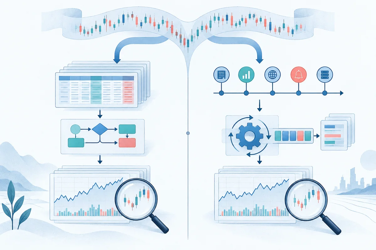
Two contrasting design philosophies in Python backtesting
Choosing between Backtrader and backtesting.py represents a fundamental architectural decision in quantitative research. While both libraries simulate strategy performance on historical price bars, they approach quantitative modeling from polar opposite software philosophies:
- Backtrader represents the comprehensive, object-oriented event-driven engine. Designed in 2015, Backtrader models a full trading ecosystem. It features an orchestration brain (
Cerebro), simulated broker accounts (Broker), line-based circular memory buffers (Lines), strategy lifecycle hooks, and extensible analyzers. It mirrors institutional event systems where orders, portfolio margins, and data feeds operate as discrete stateful entities. - backtesting.py represents the minimalist, pandas-first prototyping framework. Introduced around 2018, it intentionally strips away boilerplate. Instead of managing complex feed classes and custom line abstractions, backtesting.py consumes standard
pandas.DataFrametables directly. It provides a leaninit()andnext()strategy interface, relying on vectorized precomputation and rendering interactive HTML visual reports via Bokeh.
flowchart TD
    subgraph Backtrader ["Backtrader Event Architecture"]
        B_Data["Custom Data Feed (bt.feeds.PandasData)"] --> B_Cerebro["Cerebro Orchestrator"]
        B_Cerebro --> B_Lines["LineSeries Buffers (Relative Indexing: [0], [-1])"]
        B_Lines --> B_Strat["Strategy Instance (prenext -> nextstart -> next)"]
        B_Strat --> B_Broker["Broker Simulation (Cash, Margin, Commission)"]
        B_Broker --> B_Analyzers["Analyzers & Observers"]
    end

    subgraph BacktestingPy ["backtesting.py Procedural Architecture"]
        P_DF["Standard pandas DataFrame (Open, High, Low, Close)"] --> P_Engine["Backtest Runner"]
        P_Engine --> P_Init["Strategy.init() Vectorized Precomputation via self.I()"]
        P_Init --> P_Next["Strategy.next() Bar-by-Bar Procedural Loop"]
        P_Next --> P_Exec["Internal Order Matcher (Next-bar Open Fills)"]
        P_Exec --> P_Report["pandas.Series Metrics + Interactive Bokeh Chart"]
    end
This structural divide impacts developer ergonomics. A quant looking to rapidly validate a single-asset breakout heuristic on daily equities can configure and run a backtest in backtesting.py with fewer than 30 lines of code. Conversely, a developer requiring complex multi-data feeds, custom order execution listeners, or custom position sizing across several instruments may find backtesting.py's constraints limiting and lean toward Backtrader's modular object hierarchy.
Ingesting Data: PandasData feeds vs. DataFrame columns
How market data enters a simulation determines memory efficiency, schema flexibility, and ease of data pipeline integration.
Backtrader: bt.feeds.PandasData and LineSeries buffers
Backtrader does not execute directly on pandas DataFrames during its bar loop. Instead, it ingests a DataFrame through bt.feeds.PandasData and converts each column into an internal LineSeries object—a circular array buffer indexed relative to the current simulation time:
self.data.close[0]represents the closing price at the current bart.self.data.close[-1]represents the closing price at the prior bart-1.self.data.close[1]represents the closing price at the next bart+1(lookahead, restricted in backtesting).
import backtrader as bt
import pandas as pd

# Load raw OHLCV DataFrame
df = pd.read_csv("BTC_USD_daily.csv", index_col="timestamp", parse_dates=True)

# Feed must be wrapped in a Backtrader feed adapter
data_feed = bt.feeds.PandasData(
    dataname=df,
    datetime=None,   # Uses DataFrame index
    open="open",
    high="high",
    low="low",
    close="close",
    volume="volume",
    openinterest=-1  # Column not present in crypto/equity data
)

cerebro = bt.Cerebro()
cerebro.adddata(data_feed, name="BTC")
Because Backtrader feeds are modular objects registered with Cerebro, Backtrader natively supports multi-asset feeds. You can pass multiple PandasData instances (cerebro.adddata(data1), cerebro.adddata(data2)) and access them within strategy code via self.datas[0] and self.datas[1].
backtesting.py: Native DataFrame consumption and self.data
backtesting.py bypasses feed wrappers entirely. The Backtest runner takes a raw pandas.DataFrame as its primary input. However, it enforces a strict naming schema:
- Price column headers must be capitalized Title Case:
Open,High,Low,Close, and optionallyVolume. - Lowercase column headers (
open,close) cause an immediate runtimeValueError. - The index must be a monotonically increasing
pd.DatetimeIndex.
import pandas as pd
from backtesting import Backtest

df = pd.read_csv("BTC_USD_daily.csv", index_col="timestamp", parse_dates=True)

# Strict column formatting required
df = df.rename(columns={
    "open": "Open",
    "high": "High",
    "low": "Low",
    "close": "Close",
    "volume": "Volume"
})

# Passed directly into the Backtest constructor
# bt = Backtest(df, StrategyClass, cash=10000, commission=0.001)
Inside a strategy's next() method, data is accessed through a dynamic proxy array self.data. Unlike Backtrader's relative zero-offset, backtesting.py adopts Python array slicing conventions:
self.data.Close[-1]references the current bar (the most recent bar evaluated).self.data.Close[-2]references the previous bar.self.data.Close.sprovides access to the underlyingpandas.Seriesof prices up to the current bar.
| Data Dimension | Backtrader (bt.feeds.PandasData) | backtesting.py (pandas.DataFrame) |
|---|---|---|
| Input Type | Subclassed Feed wrapping a DataFrame or CSV | Pure pandas.DataFrame directly |
| Column Schema | Flexible; configurable column mappings in PandasData | Strict Title Case (Open, High, Low, Close) |
| Current Bar Index | self.data.close[0] | self.data.Close[-1] |
| Prior Bar Index | self.data.close[-1] | self.data.Close[-2] |
| Multi-Asset Support | Native (multiple feeds added to Cerebro) | Single-asset only (one DataFrame per backtest) |
Defining Indicators: bt.indicators vs. self.I()
Technical indicators drive algorithmic signals. The mechanisms by which Backtrader and backtesting.py calculate indicators highlight their architectural differences.
Backtrader: Declarative indicator graphs and the lifecycle
In Backtrader, indicators are declared inside the strategy's __init__() method. They are not static NumPy arrays; they are computational nodes within Cerebro's execution graph.
class DualSMA(bt.Strategy):
    params = (("fast", 10), ("slow", 30),)

    def __init__(self):
        # Declared declaratively; creates LineSeries nodes
        self.fast_sma = bt.indicators.SMA(self.data.close, period=self.params.fast)
        self.slow_sma = bt.indicators.SMA(self.data.close, period=self.params.slow)
        self.crossover = bt.indicators.CrossOver(self.fast_sma, self.slow_sma)
Backtrader automatically manages indicator warmup periods. Because a 30-period SMA requires 30 bars of data before producing a valid value, Cerebro delays invoking next() until all indicators have sufficient data:
prenext()is called for bars 1 through 29.nextstart()is called once on bar 30 when warmup finishes.next()is called for all subsequent bars.
Furthermore, Backtrader supports Line arithmetic: operators like +, -, >, and < create derived lines automatically (e.g., spread = self.fast_sma - self.slow_sma). However, writing custom indicators requires subclassing bt.Indicator and mastering Backtrader's internal meta-class system.
backtesting.py: Vectorized wrapping with self.I()
backtesting.py delegates indicator calculations to standard Python functions (NumPy, pandas, or libraries like TA-Lib) wrapped inside self.I() during Strategy.init().
def calculate_sma(series: pd.Series, period: int) -> pd.Series:
    return pd.Series(series).rolling(period).mean()

class DualSMA(Strategy):
    fast = 10
    slow = 30

    def init(self):
        # self.I runs calculate_sma once across the full array
        self.fast_sma = self.I(calculate_sma, self.data.Close.s, self.fast)
        self.slow_sma = self.I(calculate_sma, self.data.Close.s, self.slow)
self.I() precomputes the indicator across the full price vector once before the bar-by-bar loop begins. In next(), self.fast_sma exposes a sliding NumPy array view truncated at the current bar index.
[!NOTE] Unlike Backtrader's
prenext(),backtesting.pyexecutesnext()across the full bar range. Indicators returnnp.nanduring their warmup period. Functions likebacktesting.lib.crossover()handleNaNvalues gracefully, but custom logical conditions must guard againstnp.isnan(self.fast_sma[-1])to prevent unexpected evaluation failures.
Side-by-Side Code Comparison: A Dual Moving Average Strategy
To evaluate the operational differences in syntax, broker setup, and execution dispatch, let us implement the identical strategy across both engines:
- Strategy: 10-period SMA crossing over a 30-period SMA.
- Rules: Enter long 100 shares when Fast SMA crosses above Slow SMA; exit the position when Fast SMA crosses below Slow SMA.
- Initial Capital: $10,000.
- Commission: 0.1% (0.001) per trade.
Implementation 1: Backtrader
import backtrader as bt
import pandas as pd

class BacktraderDualSMA(bt.Strategy):
    params = (
        ("fast_period", 10),
        ("slow_period", 30),
        ("size", 100),
    )

    def __init__(self):
        self.fast_sma = bt.indicators.SMA(self.data.close, period=self.params.fast_period)
        self.slow_sma = bt.indicators.SMA(self.data.close, period=self.params.slow_period)
        self.crossover = bt.indicators.CrossOver(self.fast_sma, self.slow_sma)

    def next(self):
        # In Backtrader: self.position evaluates truthy if holding an open position
        if not self.position:
            if self.crossover > 0:
                self.buy(size=self.params.size)
        elif self.crossover < 0:
            self.close()

if __name__ == "__main__":
    df = pd.read_csv("historical_bars.csv", index_col=0, parse_dates=True)

    cerebro = bt.Cerebro()
    feed = bt.feeds.PandasData(dataname=df)
    cerebro.adddata(feed)
    cerebro.addstrategy(BacktraderDualSMA)

    cerebro.broker.setcash(10000.0)
    cerebro.broker.setcommission(commission=0.001)  # 0.1%

    cerebro.addanalyzer(bt.analyzers.SharpeRatio, _name="sharpe")
    cerebro.addanalyzer(bt.analyzers.DrawDown, _name="drawdown")

    results = cerebro.run()
    strat = results[0]
    print(f"Final Value: {cerebro.broker.getvalue():.2f}")
    print(f"Sharpe Ratio: {strat.analyzers.sharpe.get_analysis().get('sharperatio')}")
Implementation 2: backtesting.py
import pandas as pd
from backtesting import Backtest, Strategy
from backtesting.lib import crossover

def SMA(series: pd.Series, period: int) -> pd.Series:
    return pd.Series(series).rolling(period).mean()

class BacktestingPyDualSMA(Strategy):
    fast_period = 10
    slow_period = 30
    trade_size = 100

    def init(self):
        self.fast_sma = self.I(SMA, self.data.Close.s, self.fast_period)
        self.slow_sma = self.I(SMA, self.data.Close.s, self.slow_period)

    def next(self):
        # In backtesting.py: self.position evaluates boolean truthy if active
        if not self.position:
            if crossover(self.fast_sma, self.slow_sma):
                self.buy(size=self.trade_size)
        elif crossover(self.slow_sma, self.fast_sma):
            self.position.close()

if __name__ == "__main__":
    df = pd.read_csv("historical_bars.csv", index_col=0, parse_dates=True)
    # Ensure TitleCase schema
    df = df.rename(columns={"open": "Open", "high": "High", "low": "Low", "close": "Close"})

    bt = Backtest(
        df,
        BacktestingPyDualSMA,
        cash=10000.0,
        commission=0.001  # 0.1%
    )

    stats = bt.run()
    print(stats[["Start", "End", "Equity Final [$]", "Sharpe Ratio", "Max. Drawdown [%]"]])
Reconciling Execution and Metric Discrepancies
Researchers implementing the exact same strategy on identical data in both frameworks frequently observe differing returns, Sharpe ratios, and drawdowns. These discrepancies stem from subtle divergences in execution models, fee accounting, and statistical formulas.
1. Order fill timing: Next-bar open mechanics
Both frameworks model realistic market order execution by default: an order placed during the decision evaluation of bar t fills at the Open price of bar t+1.
However, discrepancies emerge during edge conditions:
- Cash and Margin Verification: In Backtrader, when an order is submitted at bar
t, Cerebro checks cash sufficiency immediately. At bart+1, before executing the fill at Open, the broker validates margin again. If the market gapped open higher, exhausting purchasing power, the order may be rejected. Inbacktesting.py, order sizing checks occur at fill time against remaining cash. - Price Slippage Application: Backtrader supports granular slippage configuration via
cerebro.broker.set_slippage_perc()or fixed ticks, applying slippage against the open price. Inbacktesting.py, slippage is modeled via a custom spread or modified execution price.
2. Commission calculation structures
Commission differences alter compounding equity over long backtests:
- In
backtesting.py, passingcommission=0.001strictly deducts 0.1% of the total transaction value (Price \times Quantity \times 0.001) directly from cash balance immediately upon fill. - In Backtrader,
cerebro.broker.setcommission()defaults to percentage commissions for stocks, but can also represent per-share currency fees or futures margin schedules depending on thecommtype,margin, andmultparameters. If parameters are misconfigured, Backtrader may treat0.001as $0.001 per unit rather than 0.1%.
3. Indicator warmup and start bar offsets
As demonstrated earlier, Backtrader suppresses strategy execution during the warmup window via prenext(). If the slow SMA has a period of 30, Backtrader executes its first next() call on bar 30.
In backtesting.py, next() runs starting from bar 0. While crossover() will evaluate to False while either array contains NaN, any non-indicator conditions (such as calendar filters, bar counter logic, or unhedged entries) could trigger on bars 1 through 29 in backtesting.py, generating trades that Backtrader would never take.
4. Divergent performance metric formulas
Even when identical trades occur at identical prices, the final reported summary metrics rarely match:
┌────────────────────────┬──────────────────────────────────┬─────────────────────────────────┐
│ Metric Dimension       │ Backtrader (Sharpe Analyzer)     │ backtesting.py (stats output)   │
├────────────────────────┼──────────────────────────────────┼─────────────────────────────────┤
│ Return Basis           │ Periodic returns on bar equity   │ Compounded daily equity returns │
│ Annualization Factor   │ √252 (Days), √52 (Weeks), etc.   │ √252 based on DatetimeIndex     │
│ Risk-Free Rate Subtr.  │ Per-period rate deduction        │ Fixed annualized rate default   │
│ Drawdown Tracking      │ Closed-bar or tick equity peak   │ Peak-to-trough on closed bars   │
└────────────────────────┴──────────────────────────────────┴─────────────────────────────────┘- Sharpe Ratio: Backtrader's
SharpeRatioanalyzer calculates excess periodic returns using either standard or logarithmic returns, scaled by\sqrt{252}for daily data.backtesting.pycomputes an annualized Sharpe ratio from the daily equity curve using simple returns. A difference in risk-free rate defaults or return frequency creates varying Sharpe values. - Drawdown Calculation: Backtrader records
DrawDownusing high-water mark equity across bars, reporting both maximum drawdown percentage and duration.backtesting.pyreportsMax. Drawdown [%]as the deepest single peak-to-trough decline across historical closes.
Licensing and Maintenance: AGPL-3.0 vs. GPLv3
Beyond technical mechanics, licensing and software maintenance are critical considerations for quantitative funds, corporate trading desks, and proprietary systems.
┌──────────────────────────────────┐        ┌──────────────────────────────────┐
│          backtesting.py          │        │            Backtrader            │
│             AGPL-3.0             │        │              GPLv3               │
├──────────────────────────────────┤        ├──────────────────────────────────┤
│ • Strong copyleft                │        │ • Traditional copyleft           │
│ • Network use clause (Sect. 13)  │        │ • No network use clause          │
│ • Cloud/API hosting triggers     │        │ • Dormant upstream (2019/2020)   │
│   source disclosure obligations  │        │ • Deprecations on Python 3.12+   │
└──────────────────────────────────┘        └──────────────────────────────────┘
The AGPL-3.0 constraint in backtesting.py
backtesting.py is licensed under the GNU Affero General Public License v3.0 (AGPL-3.0).
- AGPL-3.0 is a strong copyleft license with a specific network interaction clause (Section 13).
- If you run
backtesting.pywithin an internal web service, microservice API, or software-as-a-service (SaaS) platform where users or remote systems interact with the service over a network, AGPL-3.0 can trigger legal obligations to make the complete source code of the backend service available to all network users. - For proprietary trading desks, quant hedge funds, and fintech startups, AGPL-3.0 often disqualifies
backtesting.pyfrom production infrastructure.
The maintenance status of Backtrader and GPLv3
Backtrader is licensed under the GNU General Public License v3.0 (GPLv3). While GPLv3 imposes copyleft requirements upon distribution of software binaries, it does not contain the AGPL network-trigger clause.
However, Backtrader faces a significant maintenance challenge:
- The official upstream repository (
mementum/backtrader) has been largely dormant since 2019–2020. - Running vanilla Backtrader on modern Python runtimes (Python 3.12+) triggers deprecation warnings due to internal references to legacy modules (e.g.,
imp, outdatedcollections.abcconstructs). - Built-in charting via
cerebro.plot()frequently errors out on modern Matplotlib installations (\ge 3.8) due to deprecated axes and canvas attributes. - While community forks (such as
backtrader2) address specific bug fixes, the fragmentation leaves quants without an authoritative, actively maintained distribution.
Further Reading: Modern Inspectable Alternatives
As quantitative research workflows adapt to Python 3.12+ environments, engineering teams increasingly prioritize reproducibility, execution determinism, and license compatibility. Modern research platforms seek to eliminate both the metaprogramming opacity of legacy event engines and the legal friction of network copyleft licenses.
For quants evaluating current alternatives, OpenBacktesting (version 0.2.1) provides an Apache-2.0 licensed, single-asset bar-by-bar backtesting framework designed for complete auditability:
- Permissive Apache-2.0 License: Freely embeddable within internal research pipelines, microservices, and proprietary proprietary trading workflows without copyleft restrictions.
- Python 3.12+ Native: Built strictly on NumPy, pandas, and
pandas-ta-classic, avoiding legacy dependencies and meta-class overhead. - Realistic Order Lifecycle Modeling: Precise single-asset simulation supporting Market, Limit, Stop, Stop-Limit, Trailing Stop, and One-Cancels-Other (OCO) order brackets with deterministic fill mechanics.
- Durable Trial Persistence: Built-in SQLite trial persistence for parameter optimization (grid search and Sequential Adaptive Model-Based Optimization, or SAMBO), ensuring every trial, parameter combination, and execution metric is stored for retrospective analysis.
- Interactive Local Auditing: Inspect trade-by-trade logs, execution slippage, and portfolio equity paths locally via the browser-based OpenBacktesting Studio.
To explore building complete strategies with event-driven or pandas architectures, review our hands-on tutorials:
- Backtrader Tutorial: Build and Inspect Your First Strategy
- Backtesting.py Tutorial: A Complete OHLC Strategy Workflow
- OpenBacktesting Documentation
Conclusion and summary matrix
Both Backtrader and backtesting.py have made enduring contributions to Python quantitative research. Understanding their design trade-offs helps you select the appropriate tool for your specific research phase.
Head-to-head comparison matrix
| Evaluation Criteria | Backtrader | backtesting.py |
|---|---|---|
| Primary Architecture | Object-oriented event-driven engine (Cerebro) | Procedural loop over precomputed arrays |
| Input Data Format | bt.feeds.PandasData / LineSeries | Standard pandas.DataFrame (TitleCase columns) |
| Data Indexing Syntax | Relative offset (close[0], close[-1]) | Python slicing (Close[-1], Close[-2]) |
| Indicator Creation | bt.indicators computation graph | Vectorized wrappers via self.I() |
| Execution Timing | Next-bar Open fill (cheat_on_open=False) | Next-bar Open fill |
| Multi-Asset Support | Native multi-feed synchronization | Single-asset only |
| Optimization Method | Multi-core Grid Search in memory | Exhaustive Grid / Skopt Random Search |
| Trial Persistence | Ephemeral (results held in RAM) | Ephemeral (results held in RAM) |
| Visualization | Static Matplotlib chart (cerebro.plot()) | Standalone interactive Bokeh HTML |
| License | GPLv3 (Copyleft on distribution) | AGPL-3.0 (Copyleft over network/API) |
| Modern Python Support | Inactive upstream; warnings on Python 3.12+ | Stable, but pinned Bokeh dependencies |
Practical selection guide
- Choose backtesting.py if you are conducting exploratory single-asset research, require fast parameter prototyping on daily or intraday OHLCV bars, value interactive Bokeh HTML charts, and operate in an environment where AGPL-3.0 compliance is acceptable.
- Choose Backtrader if you maintain existing event-driven strategies built around
Cerebro, need native multi-asset data feeds within a single strategy instance, or require granular simulation of order states across custom brokerage observers. - Choose modern inspectable engines like OpenBacktesting if you work in Python 3.12+, require a permissive Apache-2.0 license for proprietary research, need auditable bar-by-bar execution with SQLite optimization persistence, and demand deterministic order mechanics for production-grade strategy validation.