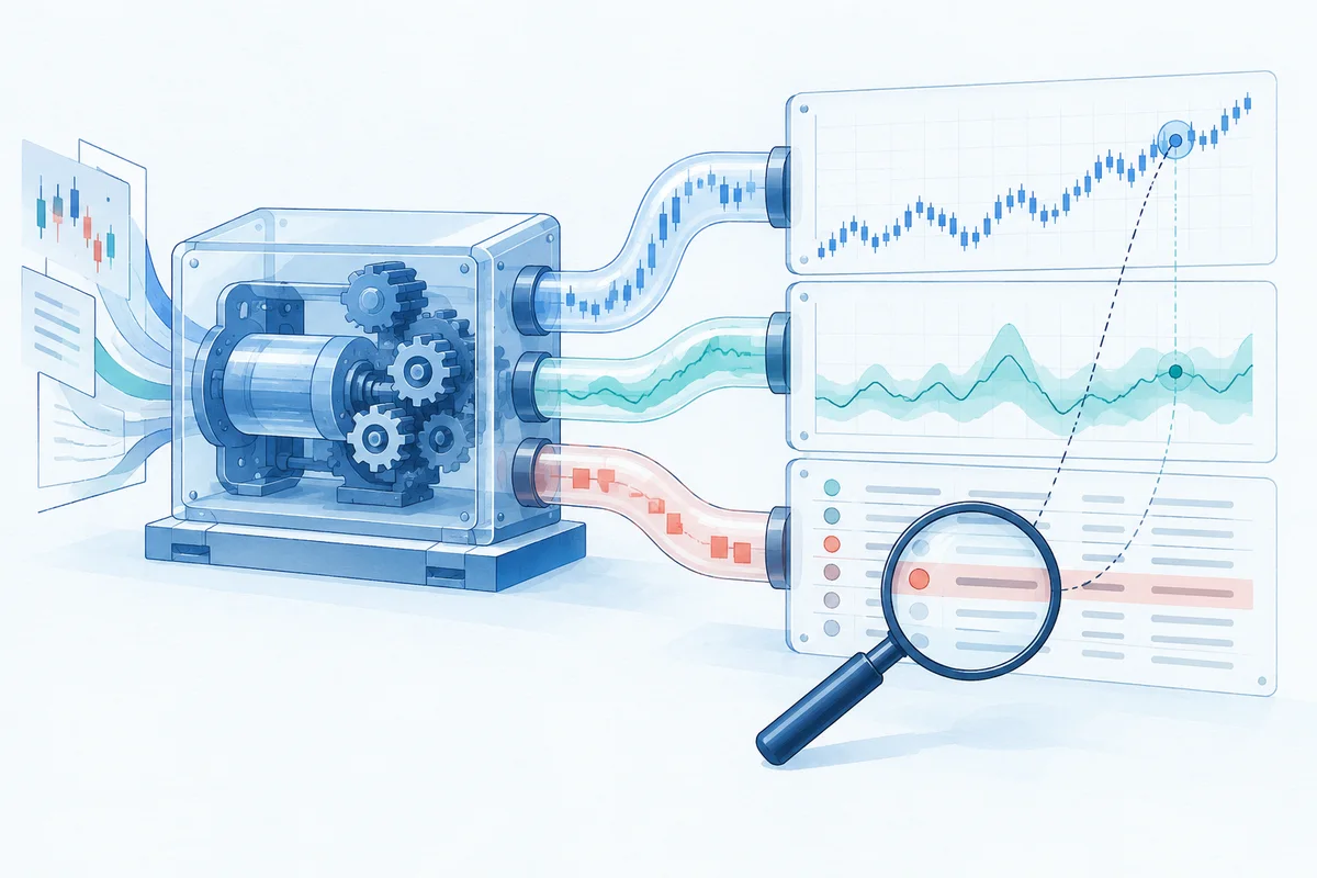
Backtrader Analyzers: Export and Audit Your Backtest Results

Beyond equity curves: Why analyzers are essential for strategy attribution

When developing quantitative trading strategies, researchers often rely on visual inspection of cumulative equity curves or raw end-of-simulation portfolio balances. Relying on an equity curve alone, however, introduces severe confirmation bias. An equity curve showing a 45% cumulative return can easily mask an intolerable 35% maximum drawdown, prolonged multi-month underwater stagnation, or extreme statistical fragility driven by a handful of outlier trades.

To determine whether an algorithmic edge is statistically genuine or merely the result of sample overfitting, quantitative researchers need rigorous strategy attribution. Attribution evaluates performance across four distinct dimensions:

Risk-Adjusted Return: Measuring excess return generated per unit of total risk (Sharpe Ratio) or downside volatility (Sortino Ratio).
Drawdown Dynamics: Quantifying peak-to-trough capital impairments, worst-case monetary loss, and time to recovery.
Trade Distribution & Efficiency: Analyzing win/loss frequencies, average win-to-loss ratios (payoff ratio), and profit factors.
Statistical Significance: Verifying that trade counts and payoff distributions satisfy baseline statistical thresholds rather than random drift.

Code

flowchart TD
    subgraph ExecutionEngine ["Cerebro Execution Engine"]
        BarData["Historical OHLCV Bars"]
        Broker["Simulated Broker (Orders / Fills / Cash)"]
        Strat["Strategy Decision Loop (next)"]
    end

    subgraph AnalyzersLayer ["Backtrader Analyzers Layer"]
        SR["SharpeRatio / SharpeRatio_A"]
        DD["DrawDown (Depth, Length, Money)"]
        TA["TradeAnalyzer (Win/Loss, PnL, Streaks)"]
        SQN["System Quality Number (SQN)"]
        TR["TimeReturn (Bar-by-Bar Returns)"]
    end

    subgraph AuditLayer ["Audit & Downstream Reporting"]
        Extract["strat.analyzers.get_analysis()"]
        Clean["AutoOrderedDict -> Flattened Dict / DataFrame"]
        Persist["Audit Ledger / JSON Reports / Quant Factsheet"]
    end

    BarData --> Strat
    Strat --> Broker
    Broker -->|"Bar & Order Events"| AnalyzersLayer
    AnalyzersLayer --> Extract
    Extract --> Clean
    Clean --> Persist

In Backtrader, this statistical extraction is handled by Analyzers (bt.Analyzer). While indicators calculate values on every bar to drive trading logic, analyzers act as non-intrusive accumulators. They observe portfolio equity, completed trades, and closed orders throughout the backtest run, aggregating raw simulation data into structured performance metrics without altering strategy execution.

Core built-in Backtrader Analyzers

Backtrader includes a suite of built-in analyzers in the bt.analyzers module. Understanding their exact calculation mechanics and configuration options is critical for accurate performance attribution.

1. `bt.analyzers.SharpeRatio` and `SharpeRatio_A`

The Sharpe ratio measures the excess return of an investment above a risk-free rate per unit of standard deviation:

Code

\text&#123;Sharpe Ratio&#125; = \frac&#123;\mathbb&#123;E&#125;[R_p - R_f]&#125;&#123;\sigma(R_p - R_f)&#125;

Backtrader provides two variations:

SharpeRatio: Computes the ratio based on periodic returns (daily, weekly, or monthly) and annualizes via a square-root scaling factor: \sqrt{K}, where K = 252 for daily equity data.
SharpeRatio_A: Directly uses annualized returns to compute the ratio.

Configuring SharpeRatio on Cerebro

cerebro.addanalyzer(
    bt.analyzers.SharpeRatio,
    _name='sharpe',
    timeframe=bt.TimeFrame.Days,
    compression=1,
    riskfreerate=0.02,     # 2.0% annual risk-free rate
    annualize=True,
    convertrate=True,      # Converts annual riskfreerate to the specified timeframe
    factor=252             # Number of trading periods per year
)

[!WARNING] The convertrate Trap: When supplying an annual risk-free rate (e.g., 0.02) on daily bars, you must pass convertrate=True. If convertrate=False, Backtrader deducts the full 2% risk-free rate from each single daily return, driving the calculated Sharpe ratio into deep negative territory. If returns have zero variance or the strategy executes no trades, get_analysis() returns {'sharperatio': None}.

2. `bt.analyzers.DrawDown`

The DrawDown analyzer monitors peak equity and evaluates relative and monetary drops. It computes two key metrics:

Current Drawdown: The active percentage and dollar drop from the prior equity high.
Max Drawdown: The historical worst peak-to-trough decline observed over the simulation.

Configuring DrawDown analyzer

cerebro.addanalyzer(bt.analyzers.DrawDown, _name='drawdown')

The output dictionary structure provides:

analysis['drawdown']: Percentage drawdown at the end of the simulation.
analysis['moneydown']: Dollar decline at the end of the simulation.
analysis['max']['drawdown']: Maximum percentage peak-to-trough decline.
analysis['max']['moneydown']: Maximum dollar loss during the worst drawdown.
analysis['max']['len']: Maximum consecutive bars spent underwater.

3. `bt.analyzers.TradeAnalyzer`

TradeAnalyzer evaluates completed, round-trip trades. It computes extensive trade attribution metrics:

Total Trades: Total, open, and closed trade counts.
Win/Loss Breakdown: Count, total PnL, average PnL, and maximum individual win or loss.
Streaks: Current and longest winning and losing streaks.
PnL Structure: Gross and net PnL (reflecting commissions and borrowing costs).
Duration: Average, maximum, and minimum bars held per trade.

4. `bt.analyzers.SQN` (System Quality Number)

Developed by Van Tharp, the System Quality Number (SQN) quantifies strategy edge by scoring the distribution of trade PnLs normalized by variance:

Code

\text&#123;SQN&#125; = \sqrt&#123;N&#125; \times \frac&#123;\bar&#123;P&#125;&#125;&#123;\sigma_P&#125;

Where N is the number of closed trades, \bar{P} is the mean trade PnL, and \sigma_P is the standard deviation of trade PnLs.

SQN Score Range	System Characterization
Below 1.6	Weak edge; statistically fragile.
1.6 – 1.9	Below average; vulnerable to market regime changes.
2.0 – 2.4	Average trading system.
2.5 – 2.9	Good, robust system edge.
3.0 – 5.0	Excellent institutional-grade system.
5.1+	Superb; inspect carefully for sample bias or lookahead leaks.

5. `bt.analyzers.TimeReturn`

The TimeReturn analyzer records the exact percentage return of portfolio value across specified time buckets (e.g., daily, monthly). Rather than summarizing results into a single scalar, it outputs an ordered time series of portfolio returns, making it the primary bridge to custom risk analytics (such as Sortino, Omega ratio, or VaR).

Configuring TimeReturn analyzer

cerebro.addanalyzer(
    bt.analyzers.TimeReturn,
    _name='timereturn',
    timeframe=bt.TimeFrame.Days
)

Built-in Analyzer Reference

Analyzer Class	Default Access Key	Primary Metric	Return Type	Common Gotcha
`SharpeRatio`	`analysis['sharperatio']`	Annualized Sharpe ratio	`float` or `None`	Returns `None` if return variance is zero or trades = 0.
`DrawDown`	`analysis['max']['drawdown']`	Peak-to-trough drop (%)	`float`	Equity drop includes open unrealized mark-to-market.
`TradeAnalyzer`	`analysis['total']['closed']`	Count of closed trades	`int`	Deeply nested `AutoOrderedDict` with missing keys on 0 trades.
`SQN`	`analysis['sqn']`	System Quality Number	`float`	Requires `\ge 30` trades for meaningful statistical power.
`TimeReturn`	`analysis[datetime_key]`	Periodic return series	`OrderedDict`	Keys are Python `datetime.date` objects.

Extracting and parsing analyzer results

Running a backtest via cerebro.run() returns a list of executed strategy instances. When a single strategy is scheduled, the strategy instance is retrieved at strat = results[0].

Code

results = cerebro.run()
strat = results[0]

The `AutoOrderedDict` serialization problem

Backtrader stores analyzer outputs in an internal data structure called bt.AutoOrderedDict (derived from collections.OrderedDict). While convenient for dynamic key insertion internally, AutoOrderedDict poses two operational headaches in production pipelines:

JSON Incompatibility: Standard json.dumps() raises TypeError: Object of type AutoOrderedDict is not JSON serializable.
Key Creation Side-Effects: Referencing a non-existent key in an AutoOrderedDict silently instantiates an empty AutoOrderedDict at that key rather than raising a KeyError.

To reliably export analyzer data to JSON, databases, or REST APIs, you must recursively clean and convert the nested structure into native Python primitives:

Recursive converter for Backtrader analyzer dictionaries

from collections import OrderedDict
import datetime
import numpy as np

def clean_analyzer_output(data):
    """
    Recursively converts AutoOrderedDict and non-primitive types 
    into standard Python dicts, floats, and ISO date strings.
    """
    if isinstance(data, (dict, OrderedDict)):
        cleaned = {}
        for key, value in data.items():
            str_key = key.isoformat() if isinstance(key, (datetime.date, datetime.datetime)) else str(key)
            cleaned[str_key] = clean_analyzer_output(value)
        return cleaned
    elif isinstance(data, (list, tuple)):
        return [clean_analyzer_output(item) for item in data]
    elif isinstance(data, (np.floating, float)):
        return None if np.isnan(data) or np.isinf(data) else float(data)
    elif isinstance(data, (np.integer, int)):
        return int(data)
    elif isinstance(data, (datetime.date, datetime.datetime)):
        return data.isoformat()
    return data

Formatting `TimeReturn` and `TradeAnalyzer` into pandas DataFrames

Downstream analysis is most efficient when converted into pandas Series or DataFrames.

Converting TimeReturn into a pandas Series

import pandas as pd

raw_returns = strat.analyzers.timereturn.get_analysis()
returns_series = pd.Series(raw_returns)
returns_series.index = pd.to_datetime(returns_series.index)
returns_series.name = "daily_returns"

# Calculate cumulative returns and drawdown series
cumulative_returns = (1.0 + returns_series).cumprod() - 1.0
peak = cumulative_returns.cummax()
drawdown_series = (cumulative_returns - peak) / (1.0 + peak)

Complete runnable code example: A comprehensive analyzer audit harness

Below is a self-contained, fully runnable script. It generates reproducible synthetic daily OHLCV bars, initializes a Simple Moving Average (SMA) crossover strategy, attaches all primary analyzers with explicit naming, executes the backtest, and prints both a formatted summary table and a validated JSON audit payload.

complete_analyzer_audit.py

import datetime
import json
from collections import OrderedDict
import backtrader as bt
import numpy as np
import pandas as pd

# ---------------------------------------------------------
# 1. Synthetic Data Generation (Reproducible Geometric Drift)
# ---------------------------------------------------------
def generate_synthetic_data(num_bars=300, seed=42):
    np.random.seed(seed)
    start_date = datetime.date(2023, 1, 1)
    date_index = [start_date + datetime.timedelta(days=i) for i in range(num_bars)]
    
    # Generate geometric Brownian motion with mild positive drift
    returns = np.random.normal(loc=0.0005, scale=0.015, size=num_bars)
    price_path = 100.0 * np.exp(np.cumsum(returns))
    
    high = price_path * (1.0 + np.random.uniform(0.002, 0.01, size=num_bars))
    low = price_path * (1.0 - np.random.uniform(0.002, 0.01, size=num_bars))
    open_p = low + (high - low) * np.random.uniform(0.2, 0.8, size=num_bars)
    close_p = low + (high - low) * np.random.uniform(0.2, 0.8, size=num_bars)
    volume = np.random.randint(50000, 200000, size=num_bars)
    
    df = pd.DataFrame({
        'open': open_p,
        'high': high,
        'low': low,
        'close': close_p,
        'volume': volume
    }, index=pd.to_datetime(date_index))
    
    return df

# ---------------------------------------------------------
# 2. Strategy Definition
# ---------------------------------------------------------
class SmaCrossStrategy(bt.Strategy):
    params = (
        ('fast_period', 10),
        ('slow_period', 30),
    )

    def __init__(self):
        self.fast_sma = bt.indicators.SMA(self.data.close, period=self.p.fast_period)
        self.slow_sma = bt.indicators.SMA(self.data.close, period=self.p.slow_period)
        self.crossover = bt.indicators.CrossOver(self.fast_sma, self.slow_sma)
        self.order = None

    def notify_order(self, order):
        if order.status in [order.Completed, order.Canceled, order.Margin, order.Rejected]:
            self.order = None

    def next(self):
        if self.order:
            return

        if not self.position:
            if self.crossover > 0:
                # Golden Cross: Enter Long
                size = int(self.broker.get_cash() * 0.95 / self.data.close[0])
                if size > 0:
                    self.order = self.buy(size=size)
        else:
            if self.crossover < 0:
                # Death Cross: Liquidate Position
                self.order = self.close()

# ---------------------------------------------------------
# 3. Serialization Helper
# ---------------------------------------------------------
def clean_dict(data):
    if isinstance(data, (dict, OrderedDict)):
        return {str(k): clean_dict(v) for k, v in data.items()}
    elif isinstance(data, (list, tuple)):
        return [clean_dict(v) for v in data]
    elif isinstance(data, (np.floating, float)):
        return None if np.isnan(data) or np.isinf(data) else round(float(data), 4)
    elif isinstance(data, (np.integer, int)):
        return int(data)
    elif isinstance(data, (datetime.date, datetime.datetime)):
        return data.isoformat()
    return data

# ---------------------------------------------------------
# 4. Engine Configuration and Execution
# ---------------------------------------------------------
def run_audit_harness():
    cerebro = bt.Cerebro()
    
    # Ingest synthetic data
    df = generate_synthetic_data(num_bars=350, seed=101)
    data = bt.feeds.PandasData(dataname=df)
    cerebro.adddata(data)
    
    # Attach strategy
    cerebro.addstrategy(SmaCrossStrategy, fast_period=10, slow_period=30)
    
    # Configure broker (Cash, Commission, Slippage)
    initial_cash = 50000.0
    cerebro.broker.setcash(initial_cash)
    cerebro.broker.setcommission(commission=0.001)  # 0.1% per trade leg
    cerebro.broker.set_slippage_perc(perc=0.0005, slip_open=True)  # 5 bps slippage
    
    # Attach Core Analyzers
    cerebro.addanalyzer(bt.analyzers.SharpeRatio, _name='sharpe', 
                        timeframe=bt.TimeFrame.Days, riskfreerate=0.0, annualize=True)
    cerebro.addanalyzer(bt.analyzers.DrawDown, _name='drawdown')
    cerebro.addanalyzer(bt.analyzers.TradeAnalyzer, _name='trades')
    cerebro.addanalyzer(bt.analyzers.SQN, _name='sqn')
    cerebro.addanalyzer(bt.analyzers.TimeReturn, _name='timereturn', timeframe=bt.TimeFrame.Days)
    
    # Execute simulation
    results = cerebro.run()
    strat = results[0]
    
    # -----------------------------------------------------
    # 5. Extract and Structure Metrics
    # -----------------------------------------------------
    sharpe_res = strat.analyzers.sharpe.get_analysis()
    dd_res = strat.analyzers.drawdown.get_analysis()
    trade_res = strat.analyzers.trades.get_analysis()
    sqn_res = strat.analyzers.sqn.get_analysis()
    
    end_val = cerebro.broker.getvalue()
    total_return_pct = ((end_val - initial_cash) / initial_cash) * 100.0
    
    total_closed = trade_res.get('total', {}).get('closed', 0)
    won_trades = trade_res.get('won', {}).get('total', 0)
    lost_trades = trade_res.get('lost', {}).get('total', 0)
    win_rate = (won_trades / total_closed * 100.0) if total_closed > 0 else 0.0
    
    pnl_net = trade_res.get('pnl', {}).get('net', {}).get('total', 0.0)
    max_dd = dd_res.get('max', {}).get('drawdown', 0.0)
    max_moneydown = dd_res.get('max', {}).get('moneydown', 0.0)
    sharpe_val = sharpe_res.get('sharperatio', None)
    sqn_val = sqn_res.get('sqn', None)
    
    audit_summary = {
        "capital": {
            "initial": initial_cash,
            "final": round(end_val, 2),
            "return_pct": round(total_return_pct, 2),
            "net_pnl": round(pnl_net, 2)
        },
        "risk": {
            "sharpe_ratio": round(sharpe_val, 3) if sharpe_val else None,
            "max_drawdown_pct": round(max_dd, 2),
            "max_drawdown_cash": round(max_moneydown, 2),
            "max_drawdown_len_bars": dd_res.get('max', {}).get('len', 0)
        },
        "trade_metrics": {
            "total_closed": total_closed,
            "won": won_trades,
            "lost": lost_trades,
            "win_rate_pct": round(win_rate, 2),
            "sqn": round(sqn_val, 2) if sqn_val else None
        }
    }
    
    print("=================== STRATEGY AUDIT REPORT ===================")
    print(f"Ending Value:      ${audit_summary['capital']['final']:,.2f} ({audit_summary['capital']['return_pct']}%)")
    print(f"Net Realized PnL:  ${audit_summary['capital']['net_pnl']:,.2f}")
    print(f"Sharpe Ratio:      {audit_summary['risk']['sharpe_ratio']}")
    print(f"Max Drawdown:      {audit_summary['risk']['max_drawdown_pct']}% (${audit_summary['risk']['max_drawdown_cash']:,.2f})")
    print(f"Underwater Length: {audit_summary['risk']['max_drawdown_len_bars']} bars")
    print(f"Closed Trades:     {audit_summary['trade_metrics']['total_closed']} (Win Rate: {audit_summary['trade_metrics']['win_rate_pct']}%)")
    print(f"System Quality:    SQN {audit_summary['trade_metrics']['sqn']}")
    print("=============================================================")
    
    # Clean and dump full JSON audit payload
    raw_payload = {
        "summary": audit_summary,
        "raw_drawdown": clean_dict(dd_res),
        "raw_trades": clean_dict(trade_res),
        "raw_sqn": clean_dict(sqn_res)
    }
    
    json_output = json.dumps(raw_payload, indent=2)
    with open("strategy_audit_export.json", "w") as f:
        f.write(json_output)
    print("Successfully exported JSON audit payload to 'strategy_audit_export.json'.")

if __name__ == '__main__':
    run_audit_harness()

Authoring a custom Analyzer subclass

While built-in analyzers capture standard metrics, quantitative production requirements frequently require custom calculations such as Profit Factor, Calmar Ratio, or R-multiple distributions.

The `bt.Analyzer` lifecycle

Subclassing bt.Analyzer requires implementing specific lifecycle hooks:

Code

flowchart TD
    Init["__init__()\nDeclare parameters & storage"] --> Start["start()\nInvoked before bar 0"]
    Start --> BarLoop["Bar Iteration Loop"]
    BarLoop --> Next["next() / notify_cashvalue()\nEvaluate equity & active risk"]
    BarLoop --> OrderNotify["notify_order(order)\nTrack order fills & commissions"]
    BarLoop --> TradeNotify["notify_trade(trade)\nRecord round-trip PnL & duration"]
    BarLoop --> Stop["stop()\nCompute final summary metrics"]
    Stop --> GetAnalysis["get_analysis()\nExpose final results dict"]

start(): Called once immediately before Cerebro begins processing bars. Initialize counters, tracking lists, and dictionaries here.
notify_order(order): Invoked whenever an order status updates. Useful for tracking commission drag, rejected orders, or fill slippage.
notify_trade(trade): Invoked whenever an existing trade position is closed or updated. When trade.isclosed is True, the trade's realized gross PnL (trade.pnl), net PnL (trade.pnlcomm), duration in bars (trade.barlen), and timestamps are accessible.
notify_cashvalue(cash, value): Invoked on every bar tick with current free cash and portfolio net asset value.
stop(): Invoked once when all bars have been processed. Finalize aggregate calculations and store them inside self.rets.
get_analysis(): By default, returns self.rets. You can override this method to return custom dictionaries or DataFrames.

Implementation: Building a `TradeAuditAnalyzer`

Here is an implementation of a custom analyzer that calculates the Profit Factor, separates gross gains and losses, records trade durations, and computes the average win-to-loss ratio (Payoff Ratio):

Code

\text&#123;Profit Factor&#125; = \frac&#123;\sum \text&#123;Gross Wins&#125;&#125;&#123;|\sum \text&#123;Gross Losses&#125;|&#125;

Code

\text&#123;Payoff Ratio&#125; = \frac&#123;\text&#123;Mean Win PnL&#125;&#125;&#123;|\text&#123;Mean Loss PnL&#125;|&#125;

custom_trade_auditor.py

import backtrader as bt
import numpy as np

class TradeAuditAnalyzer(bt.Analyzer):
    """
    Custom Analyzer tracking Profit Factor, Payoff Ratio,
    trade holding periods, and full round-trip trade ledgers.
    """
    params = (
        ('risk_free_rate', 0.0),
    )

    def start(self):
        super().start()
        self.trades = []
        self.wins = []
        self.losses = []

    def notify_trade(self, trade):
        # We only record closed round-trips
        if not trade.isclosed:
            return

        gross_pnl = trade.pnl
        net_pnl = trade.pnlcomm
        commission = gross_pnl - net_pnl
        bars_held = trade.barlen

        trade_record = {
            'ref': trade.ref,
            'dtopen': bt.num2date(trade.dtopen).isoformat(),
            'dtclose': bt.num2date(trade.dtclose).isoformat(),
            'bars_held': bars_held,
            'gross_pnl': round(gross_pnl, 2),
            'net_pnl': round(net_pnl, 2),
            'commission': round(commission, 2)
        }
        self.trades.append(trade_record)

        if net_pnl > 0:
            self.wins.append(net_pnl)
        elif net_pnl < 0:
            self.losses.append(abs(net_pnl))

    def stop(self):
        super().stop()
        total_closed = len(self.trades)
        sum_wins = sum(self.wins)
        sum_losses = sum(self.losses)

        # Profit Factor calculation
        if sum_losses > 0:
            profit_factor = sum_wins / sum_losses
        elif sum_wins > 0:
            profit_factor = float('inf')
        else:
            profit_factor = 0.0

        # Payoff Ratio calculation
        mean_win = float(np.mean(self.wins)) if self.wins else 0.0
        mean_loss = float(np.mean(self.losses)) if self.losses else 0.0
        payoff_ratio = (mean_win / mean_loss) if mean_loss > 0 else 0.0

        # Holding duration
        durations = [t['bars_held'] for t in self.trades]
        avg_bars_held = float(np.mean(durations)) if durations else 0.0

        self.rets['total_trades'] = total_closed
        self.rets['profit_factor'] = round(profit_factor, 3)
        self.rets['payoff_ratio'] = round(payoff_ratio, 3)
        self.rets['avg_bars_held'] = round(avg_bars_held, 1)
        self.rets['gross_wins_sum'] = round(sum_wins, 2)
        self.rets['gross_losses_sum'] = round(sum_losses, 2)
        self.rets['trade_ledger'] = self.trades

    def get_analysis(self):
        return self.rets

To register and use this analyzer in your strategy:

Code

cerebro.addanalyzer(TradeAuditAnalyzer, _name='custom_audit')
results = cerebro.run()
audit = results[0].analyzers.custom_audit.get_analysis()

print(f"Profit Factor: {audit['profit_factor']}")
print(f"Payoff Ratio:  {audit['payoff_ratio']}")
print(f"Avg Duration:  {audit['avg_bars_held']} bars")

Modern auditing vs. legacy analyzers

Backtrader's analyzer design was progressive when introduced in 2015. However, maintaining large-scale research pipelines reveals architectural limitations inherent to legacy Python frameworks.

The challenges of Backtrader's analyzer architecture

Coupled Execution State: Analyzers depend directly on Backtrader's OOP metaclass hierarchy. Extracting data requires instantiating the entire Cerebro engine and stepping through custom LineSeries iterators.
In-Memory Volatility: During parameter optimization (cerebro.optstrategy), Backtrader stores every completed strategy and analyzer instance in Python process memory. For large parameter sweeps (e.g., 5,000+ combinations), this frequently causes Out-Of-Memory (OOM) crashes unless users write manual file dumpers.
Complex Deserialization: Because analyzers return nested AutoOrderedDict instances containing mixins of datetime objects, floats, and internal references, quants must write extensive custom parsing scripts just to export clean trade logs into compliance-ready formats.

The OpenBacktesting approach: Immutable DataFrames and SQLite trial persistence

In modern quantitative frameworks like OpenBacktesting (v0.2.1), auditing is designed around immutable columnar data structures rather than mutable event dictionaries.

OpenBacktesting operates as a single-asset historical OHLCV bar-by-bar backtesting engine built on Python >=3.12, <3.15, with core dependencies limited to NumPy, pandas, and pandas-ta-classic.

Code

flowchart LR
    subgraph Backtrader ["Legacy: Backtrader"]
        BT_Run["cerebro.run()"] --> BT_Opt["In-Memory Strategy List"]
        BT_Opt --> BT_AOD["AutoOrderedDict Hierarchy"]
        BT_AOD --> BT_Script["Manual JSON / DF Parsing Script"]
    end

    subgraph OpenBacktesting ["Modern: OpenBacktesting (v0.2.1)"]
        OBT_Run["backtest.run()"] --> OBT_Ledger["Immutable Ledger (_trades, _orders)"]
        OBT_Ledger --> OBT_Report["Portfolio Report & Metric Summary"]
        OBT_Report --> OBT_SQL["Native SQLite Trial Persistence"]
        OBT_SQL --> OBT_Studio["Local OpenBacktesting Studio"]
    end

Dimension	Backtrader (Legacy)	OpenBacktesting (v0.2.1)
Execution Architecture	Event-driven OOP state machine (`Cerebro`)	Bar-by-bar procedural loop with strict lookahead guards
Trade Ledger Output	Nested `AutoOrderedDict` inside `TradeAnalyzer`	Immutable pandas DataFrame (`portfolio.trades_df`)
Order Ledger Output	Manual interception via `notify_order()`	Immutable pandas DataFrame (`portfolio.orders_df`)
Parameter Sweep Storage	Ephemeral in-memory strategy references	Native SQLite trial persistence (Grid & SAMBO Bayesian search)
Interactive Inspection	Legacy Matplotlib GUI (`cerebro.plot()`)	Local browser-based OpenBacktesting Studio
Dependencies	Custom framework core, legacy Matplotlib	Modern lean core: Python `\ge 3.12`, NumPy, pandas, `pandas-ta-classic`

In OpenBacktesting, when a backtest run concludes:

Every order submission, slippage deduction, and fill timestamp is saved into an immutable order ledger.
Trade statistics (entry price, exit price, holding period, gross return, net return) are directly accessible as standard pandas DataFrames.
Optimization trials are committed incrementally to an SQLite database file. If an optimization sweep is interrupted, existing trials are fully preserved and queryable using standard SQL or pandas queries.

Summary checklist for analyzer auditing

Before deploying strategy research or publishing performance findings, audit your analyzer configurations against this verification checklist:

Risk-free rate frequency matching: If your data feed uses daily bars, ensure convertrate=True is enabled when configuring bt.analyzers.SharpeRatio, or provide a pre-converted daily risk-free rate.
Annualization factor correctness: Confirm that factor=252 is set for standard equities/bonds, factor=365 for 24/7 crypto markets, or factor=260 for 5-day forex markets.
Statistical trade sample size: Require at least 30–50 completed round-trip trades before interpreting Sharpe Ratio or SQN. Systems with fewer than 20 trades exhibit extreme standard error.
Slippage and commission inclusion: Check that analysis['pnl']['net']['total'] is evaluated rather than analysis['pnl']['gross']['total']. Zero-slippage and zero-commission backtests produce non-replicable metrics.
Serialization safety: Ensure recursive conversion wrappers are applied to AutoOrderedDict instances before passing results to standard logging or JSON file writers.
Outlier robustness audit: Remove the top 2% of winning trades and re-evaluate whether the strategy remains profitable. A strategy dependent on 1 or 2 outlier wins has poor distribution stability.

Backtrader Tutorial: Build and Inspect Your First Strategy — Core guide to Cerebro mechanics, LineSeries, and strategy lifecycle hooks.
Backtrader Sharpe Ratio: Daily vs Annualized Configuration — Deep dive into risk-free rate conversions and annualization pitfalls in Backtrader.
Profit Factor in Backtesting: Mathematics and Audit Techniques — Detailed mathematical breakdown of win/loss distribution metrics.
Maximum Drawdown in Python: Calculation, Duration, and Recovery — Comprehensive analysis of peak-to-trough risk metrics.
OpenBacktesting Documentation — Official documentation for modern bar-by-bar strategy backtesting, execution modeling, and SQLite parameter persistence.

Beyond equity curves: Why analyzers are essential for strategy attributionCopy Anchor Link

Core built-in Backtrader AnalyzersCopy Anchor Link

1. bt.analyzers.SharpeRatio and SharpeRatio_ACopy Anchor Link

2. bt.analyzers.DrawDownCopy Anchor Link

3. bt.analyzers.TradeAnalyzerCopy Anchor Link

4. bt.analyzers.SQN (System Quality Number)Copy Anchor Link

5. bt.analyzers.TimeReturnCopy Anchor Link

Built-in Analyzer ReferenceCopy Anchor Link

Extracting and parsing analyzer resultsCopy Anchor Link

The AutoOrderedDict serialization problemCopy Anchor Link

Formatting TimeReturn and TradeAnalyzer into pandas DataFramesCopy Anchor Link

Complete runnable code example: A comprehensive analyzer audit harnessCopy Anchor Link

Authoring a custom Analyzer subclassCopy Anchor Link

The bt.Analyzer lifecycleCopy Anchor Link

Implementation: Building a TradeAuditAnalyzerCopy Anchor Link

Modern auditing vs. legacy analyzersCopy Anchor Link

The challenges of Backtrader's analyzer architectureCopy Anchor Link

The OpenBacktesting approach: Immutable DataFrames and SQLite trial persistenceCopy Anchor Link

Summary checklist for analyzer auditingCopy Anchor Link

Further reading and related resourcesCopy Anchor Link

Beyond equity curves: Why analyzers are essential for strategy attribution

Core built-in Backtrader Analyzers

1. `bt.analyzers.SharpeRatio` and `SharpeRatio_A`

2. `bt.analyzers.DrawDown`

3. `bt.analyzers.TradeAnalyzer`

4. `bt.analyzers.SQN` (System Quality Number)

5. `bt.analyzers.TimeReturn`

Built-in Analyzer Reference

Extracting and parsing analyzer results

The `AutoOrderedDict` serialization problem

Formatting `TimeReturn` and `TradeAnalyzer` into pandas DataFrames

Complete runnable code example: A comprehensive analyzer audit harness

Authoring a custom Analyzer subclass

The `bt.Analyzer` lifecycle

Implementation: Building a `TradeAuditAnalyzer`

Modern auditing vs. legacy analyzers

The challenges of Backtrader's analyzer architecture

The OpenBacktesting approach: Immutable DataFrames and SQLite trial persistence

Summary checklist for analyzer auditing

Further reading and related resources