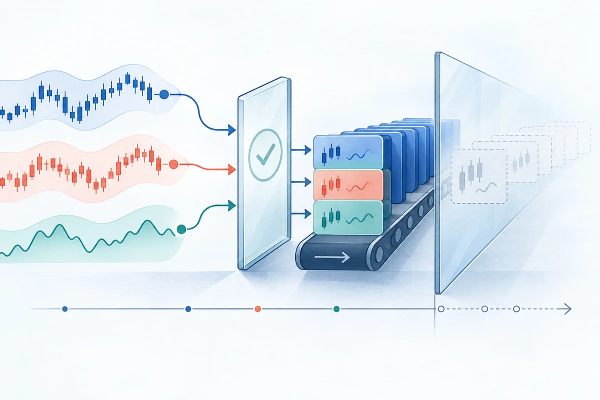
Expanding beyond OHLCV: The need for alternative data
In quantitative strategy research, standard open, high, low, close, and volume (OHLCV) bars represent only a partial slice of market dynamics. While technical indicators computed exclusively from price action—such as moving average crossovers, RSI, and Bollinger Bands—remain popular benchmarks, modern systematic alpha models increasingly rely on exogenous, non-price information streams.
Quantitative researchers incorporate diverse alternative datasets to capture regime switches, market sentiment, and positioning imbalances before they fully reflect in standard price bars:
- Sentiment Signals: Natural language processing (NLP) scores derived from financial news headlines, earnings call transcripts, regulatory filings, or social media velocity (e.g., retail discussion volume).
- Options and Volatility Surfaces: Exogenous implied volatility indices (such as the CBOE VIX), put/call ratios, options skew, and volatility risk premia.
- Market Microstructure & Crypto Positioning: Perpetual swap funding rates, open interest drift, liquidation aggregates, and order book bid-ask imbalance metrics.
- Macroeconomic Prints: Point-in-time releases of the Consumer Price Index (CPI), Non-Farm Payrolls (NFP), Federal Reserve interest rate decisions, and Purchasing Managers' Index (PMI) readings.
Standard OHLCV Bar Feed
┌────────────┬─────────┬─────────┬─────────┬─────────┬──────────┐
│  DateTime  │  Open   │  High   │   Low   │  Close  │  Volume  │
└─────┬──────┴────┬────┴────┬────┴────┬────┴────┬────┴────┬─────┘
      │           │         │         │         │         │
      ▼           ▼         ▼         ▼         ▼         ▼
┌───────────────────────────────────────────────────────────────┐
│               Exogenous Data Layer (Alternative)              │
│  • Sentiment Score [-1.0, 1.0]                                │
│  • Perpetual Funding Rate (bps)                               │
│  • 30-Day Implied Volatility (IV)                             │
└───────────────────────────────┬───────────────────────────────┘
                                │
                                ▼
┌───────────────────────────────────────────────────────────────┐
│              Strategy Decision Engine (Bar t Close)           │
│   Enter Long iff: Close > SMA(50) AND Sentiment > 0.50        │
│                   AND Funding Rate < -0.01%                   │
└───────────────────────────────────────────────────────────────┘
The challenge for algorithmic researchers lies in data ingestion. Backtesting engines designed around traditional price series assume a rigid tabular schema: a datetime index coupled with five numeric columns. In Backtrader, the built-in bt.feeds.PandasData and bt.feeds.GenericCSVData classes natively understand only standard price attributes (Open, High, Low, Close, Volume, OpenInterest).
To incorporate exogenous columns, quants must extend Backtrader's internal line buffer system. However, passing additional data columns into an event-driven backtest introduces severe structural hazards: temporal misalignment and lookahead leakage. Without strict causal synchronization, an alternative feature can silently inject future information into bar-level decision logic, invalidating backtest results.
Architecture of custom feeds in Backtrader
Backtrader's core architecture relies on an abstraction called Lines. A LineSeries is a multidimensional array-like buffer that streams time-series values bar by bar. Standard feeds implement five core lines: open, high, low, close, and volume.
When working with pandas.DataFrame objects, Backtrader provides bt.feeds.PandasData. Extending this class to ingest custom fields requires understanding two class-level declarations: lines and params.
Metaclass inheritance: lines and params
Backtrader uses Python metaclasses (MetaPandasData and MetaLineSeries) to construct class structures at import time. When you declare attributes inside a PandasData subclass, the metaclass dynamically creates internal memory buffers, descriptor getters, and iterator handles.
import backtrader as bt

class ExtendedPandasData(bt.feeds.PandasData):
    # 1. Define new lines to be created in the line buffer
    lines = ('sentiment', 'funding_rate', 'iv')

    # 2. Map line names to DataFrame column names or positional column indices
    params = (
        ('sentiment', -1),
        ('funding_rate', -1),
        ('iv', -1),
    )
Parameter mapping conventions
The params tuple defines how Backtrader matches lines to columns in the incoming pandas DataFrame:
| Parameter Value | Resolution Mechanism | Example |
|---|---|---|
-1 | Auto-detect: Backtrader searches the DataFrame for a column matching the line name (case-insensitive string match). | ('sentiment', -1) matches df['sentiment'] or df['Sentiment']. |
None | Disabled: The line is declared but not populated from the DataFrame; values default to float('nan'). | ('iv', None) skips column loading. |
Integer (>= 0) | Positional index: Resolves the column by its zero-based numerical index in the DataFrame. | ('funding_rate', 5) maps the 6th column to funding_rate. |
String | Explicit column label: Maps the line to an exact DataFrame column name, useful when names diverge. | ('sentiment', 'news_polarity_score'). |
[!IMPORTANT] When subclassing
bt.feeds.PandasData, do not redefine existing standard lines (open,high,low,close,volume,openinterest). Backtrader automatically inherits standard parameters frombt.feeds.PandasData.params. Only define the delta (the new custom lines) in your subclasslinestuple.
Access patterns inside the strategy
Once loaded into Backtrader's Cerebro engine, custom lines are accessible through identical syntax to standard price lines:
class ExogenousDataStrategy(bt.Strategy):
    def next(self):
        # Current bar value (bar t)
        current_sentiment = self.data.sentiment[0]
        current_funding = self.data.funding_rate[0]

        # Previous bar value (bar t-1)
        prev_sentiment = self.data.sentiment[-1]

        # Access via explicit data feed index
        raw_iv = self.datas[0].iv[0]
Furthermore, Backtrader's indicator library can operate directly on custom lines. For example, calculating a 5-period simple moving average of a sentiment score is fully supported:
self.sentiment_ma = bt.indicators.SMA(self.data.sentiment, period=5)Internal limitations and constraints
While Backtrader's line extension mechanism is functional, quantitative engineers must remain mindful of three architectural limitations:
- C-Level Float Buffers: Backtrader lines are backed by fixed-type floating-point array structures. They cannot store arbitrary Python objects, strings, booleans, or nested dictionaries. Any non-numeric string passed in a custom DataFrame column will trigger a
TypeError: float() argument must be a string or a real number. - Strict Index Homogeneity: If you pass multiple data feeds into
Cerebro(e.g., an equity price feed and an exogenous sentiment feed), Backtrader synchronizes them via datetime timestamps. If an exogenous feed contains missing timestamps or mismatched timezone offsets, Backtrader will skip bars or freeze indicator calculation buffers unexpectedly. - Metaclass Opacity: Errors stemming from misspelled parameter mappings or line collisions do not fail with clear exceptions; they often surface as silent
NaNpropagation or crypticIndexError: array index out of rangefailures deep withinlineiterator.py.
The danger of temporal misalignment and future leakage
Extending a data feed is straightforward syntactically, but mathematically dangerous. Alternative data feeds are the single largest source of lookahead bias (future leakage) in quantitative strategy research.
flowchart TD
    subgraph Lookahead Bias Mechanism
        A["Alternative Data Event\n(e.g., Daily Sentiment Aggregation)"] -->|Calculated at 23:59 UTC| B["Data Tagged as '2026-08-08'"]
        B -->|Blind Merge by Date| C["Daily Price Bar '2026-08-08'\n(Closes at 16:00 EST / 21:00 UTC)"]
        C -->|Strategy next() executes| D["Signal generated at 16:00 EST\nusing Sentiment from 23:59 UTC!"]
        D --> E["Lookahead Leakage: 3 Hours of Future Information!"]
    end
1. Point-in-time publication delays vs. Bar close
Financial markets operate on strict chronological causality. An algorithm making a trading decision at bar close t may only observe information that was publicly accessible at or before t.
Consider three real-world alternative data sources:
- Macroeconomic Announcements (CPI / NFP): The US CPI report is published at 08:30:00 EST. If you backtest on daily bars where the timestamp represents the trading day (
2026-08-08 00:00:00), merging the CPI print onto the day's record allows the backtest to trade at the market open (09:30:00 EST) with knowledge of the report—even if your raw data file merely lists the date without a timestamp. - Aggregated Social/News Sentiment: Many data vendors aggregate sentiment over a 24-hour UTC window and assign the record a date stamp of
YYYY-MM-DD. However, a daily equity bar closes at 16:00:00 EST (21:00:00 UTC). If you evaluateself.data.sentiment[0]on the close of that daily bar, your strategy evaluates sentiment accumulated between 21:00:00 UTC and 23:59:59 UTC—three hours into the future. - Crypto Perpetual Funding Rates: Perpetual funding is settled periodically (typically every 8 hours at 00:00, 08:00, and 16:00 UTC). A funding rate applied to a 1-hour bar series must account for whether the rate is an estimated real-time premium or the finalized historical settlement rate. Using a settlement rate finalized at 08:00:00 UTC to execute a trade at 07:30:00 UTC is direct future leakage.
2. The forward-filling (ffill()) hazard
Because alternative data arrives at irregular intervals (e.g., sporadic SEC 10-Q filings, analyst earnings revisions, or discrete macroeconomic prints), quants frequently resample or reindex the series to match high-frequency OHLCV bars using forward-fill:
# DANGEROUS: If macro_df timestamps represent publication completion,
# blind reindexing without accounting for dissemination latency leaks future data.
aligned_df = macro_df.reindex(price_df.index).ffill()
If an event occurred at 10:02:15, and the price bars are 5-minute bars labeled at interval start (10:00:00), a naive forward-fill maps the 10:02:15 event into the 10:00:00 bar. Any signal calculated at the 10:00:00 bar now executes with data that occurred two minutes later.
3. The timestamp semantics dilemma
To guarantee causal validity, you must resolve the semantic meaning of your timestamps:
\text{Timestamp Semantics} = \begin{cases}
\text{Left-labeled (Interval Start):} & [t, t + \Delta t) \\
\text{Right-labeled (Interval Close):} & (t - \Delta t, t]
\end{cases}
If your price bars are right-labeled (e.g., standard daily bars dated at market close) and your alternative data feed is left-labeled (dated at the start of the measurement window), merging on index guarantees a 1-bar lookahead bias across every trade.
[!WARNING] The Golden Rule of Causal Synchronization: An alternative data feature
Xwith publication timestamp\tau_{\text{pub}}and dissemination latency\Delta_{\text{latency}}can only be accessed on price bartif:
\tau_{\text{pub}} + \Delta_{\text{latency}} \le \tau_{\text{bar\_close}}(t)If there is any ambiguity regarding the exact publication minute of a daily alternative data metric, you must defensively apply
.shift(1)to lag the entire feature series by one full bar.
Complete runnable Python example
The following self-contained Python script demonstrates how to construct a custom Backtrader data feed extending bt.feeds.PandasData. It generates synthetic daily price data alongside two exogenous signals: sentiment (a bounded oscillator) and funding_rate (basis points).
To eliminate lookahead bias, exogenous signals are explicitly lagged by one day (.shift(1)), ensuring that the strategy's decision at the close of bar t only evaluates information that had finalized prior to the bar's open.
import datetime
import numpy as np
import pandas as pd
import backtrader as bt


# =====================================================================
# 1. Generate Synthetic Data with Exogenous Features
# =====================================================================
def create_synthetic_data(num_bars: int = 150) -> pd.DataFrame:
    np.random.seed(42)
    start_date = datetime.date(2026, 1, 1)
    dates = [start_date + datetime.timedelta(days=i) for i in range(num_bars)]

    # Generate geometric Brownian motion for price
    returns = np.random.normal(loc=0.0005, scale=0.018, size=num_bars)
    price = 100.0 * np.exp(np.cumsum(returns))

    high = price * (1.0 + np.abs(np.random.normal(0, 0.008, num_bars)))
    low = price * (1.0 - np.abs(np.random.normal(0, 0.008, num_bars)))
    open_p = price * (1.0 + np.random.normal(0, 0.004, num_bars))
    volume = np.random.randint(50000, 250000, size=num_bars).astype(float)

    # Exogenous Signal 1: Raw Sentiment (-1.0 to +1.0)
    raw_sentiment = np.clip(np.random.normal(0.05, 0.4, size=num_bars), -1.0, 1.0)

    # Exogenous Signal 2: Perpetual Funding Rate in basis points (-0.05% to +0.05%)
    raw_funding = np.random.normal(0.0001, 0.0003, size=num_bars)

    df = pd.DataFrame({
        'open': open_p,
        'high': high,
        'low': low,
        'close': price,
        'volume': volume,
        'openinterest': 0.0,
        # RAW UNFILTERED EXOGENOUS SIGNALS:
        'raw_sentiment': raw_sentiment,
        'raw_funding': raw_funding,
    }, index=pd.to_datetime(dates))

    # =================================================================
    # CRITICAL: Causal alignment via explicit shift.
    # A sentiment or funding score calculated over the course of day t
    # cannot be known until day t ends. Therefore, it is shifted forward
    # by 1 bar so that day t+1 trades on finalized day t data.
    # =================================================================
    df['sentiment'] = df['raw_sentiment'].shift(1)
    df['funding_rate'] = df['raw_funding'].shift(1)

    # Drop initial NaN introduced by the shift
    df = df.dropna()
    return df


# =====================================================================
# 2. Subclass bt.feeds.PandasData to Declare Custom Lines
# =====================================================================
class AlternativePandasData(bt.feeds.PandasData):
    """
    Extends Backtrader's PandasData feed to ingest custom lines:
    - sentiment: News / social media sentiment score [-1.0, 1.0]
    - funding_rate: Perpetual swap 8h funding rate
    """
    # Declare the additional lines
    lines = ('sentiment', 'funding_rate')

    # Map lines to DataFrame column headers (-1 means auto-match column name)
    params = (
        ('sentiment', -1),
        ('funding_rate', -1),
    )


# =====================================================================
# 3. Define Strategy Ingesting Custom Lines
# =====================================================================
class AlternativeDataStrategy(bt.Strategy):
    params = (
        ('sentiment_threshold', 0.20),
        ('sma_period', 15),
    )

    def __init__(self):
        # Built-in indicator on price
        self.sma = bt.indicators.SMA(self.data.close, period=self.params.sma_period)

        # Built-in indicator applied directly to the custom 'sentiment' line!
        self.sentiment_ma = bt.indicators.SMA(self.data.sentiment, period=5)

    def next(self):
        # Extract values at current bar close (t)
        dt = self.data.datetime.date(0)
        close_price = self.data.close[0]
        sent_val = self.data.sentiment[0]
        funding_val = self.data.funding_rate[0]
        sma_val = self.sma[0]

        # Verify alignment: print diagnostic bar information
        # print(f"[{dt}] Close: {close_price:.2f} | Sent: {sent_val:.3f} | Funding: {funding_val:.5f}")

        if not self.position:
            # Long Entry Condition:
            # Price > SMA AND Sentiment positive & rising AND Funding rate negative (discount)
            if (close_price > sma_val and
                sent_val > self.params.sentiment_threshold and
                sent_val > self.sentiment_ma[0] and
                funding_val < 0.0):

                self.order = self.buy(size=100)
                # print(f"[{dt}] BUY ORDER CREATED @ Close {close_price:.2f}")
        else:
            # Exit Condition:
            # Sentiment deteriorates below neutral or price breaks SMA
            if sent_val < 0.0 or close_price < sma_val:
                self.order = self.close()
                # print(f"[{dt}] EXIT ORDER CREATED @ Close {close_price:.2f}")


# =====================================================================
# 4. Configure Engine and Run Backtest
# =====================================================================
def run_custom_feed_backtest():
    cerebro = bt.Cerebro()
    cerebro.broker.setcash(100000.0)
    cerebro.broker.setcommission(commission=0.001)  # 10 bps commission

    # Configure 0.05% execution slippage
    cerebro.broker.set_slippage_perc(perc=0.0005, slip_open=True, slip_match=True)

    # Prepare data
    df = create_synthetic_data(num_bars=200)

    # Load custom feed into Backtrader
    data_feed = AlternativePandasData(dataname=df)
    cerebro.adddata(data_feed)

    # Add strategy
    cerebro.addstrategy(AlternativeDataStrategy)

    print(f"Starting Portfolio Value: ${cerebro.broker.getvalue():,.2f}")
    cerebro.run()
    print(f"Final Portfolio Value:    ${cerebro.broker.getvalue():,.2f}")


if __name__ == '__main__':
    run_custom_feed_backtest()
Script execution mechanics
- Explicit Causal Lag (
df['sentiment'] = df['raw_sentiment'].shift(1)): The raw sentiment score generated over the course of daytis strictly shifted to dayt+1. WhenAlternativeDataStrategy.next()evaluatesself.data.sentiment[0]on dayt+1, it accesses finalized data from dayt. - Schema Declaration (
AlternativePandasData): Declareslines = ('sentiment', 'funding_rate'). The-1parameters instruct Backtrader to automatically locate the'sentiment'and'funding_rate'columns in the pandas DataFrame. - Line Indicator Composition (
bt.indicators.SMA(self.data.sentiment, period=5)): Demonstrates Backtrader's line polymorphism, allowing moving averages, smoothed filters, or rate-of-change indicators to be stacked on exogenous lines just as easily as on price lines. - Execution Modeling: Realistic slippage (
cerebro.broker.set_slippage_perc) and commissions are applied, ensuring that signals reacting to volatile alternative data are subjected to realistic friction.
Modern approaches to multi-feature data contracts
While Backtrader's line system was pioneering upon its release in 2015, quantitative engineering practices have matured. Modern backtesting workflows prioritize explicit data contracts, typed tabular dataframes, transparent execution semantics, and zero metaclass overhead.
Limitations of Backtrader's metaclass model
Backtrader relies extensively on Python metaclass inheritance (MetaParams, MetaLineSeries, MetaPandasData) to achieve domain-specific line syntax. However, this design imposes significant developer overhead:
- Metaclass Opacity & Rigidity: Adding ten alternative signals requires modifying custom class definitions and maintaining nested parameter tuples. It is impossible to dynamically append a feature column from a DataFrame at runtime without subclassing.
- Strict Float-Only Constraints: In machine learning and factor modeling, strategies often consume string tokens (e.g., regime labels such as
'HIGH_VOL'or'TRENDING'), categorical tags, or boolean masks. Backtrader cannot store non-float types inside its line buffers. - Obscure Debugging: When a column name is misspelled or missing from the DataFrame, Backtrader does not raise a descriptive validation error at data load; it often fails downstream during iteration with cryptic tracebacks.
The OpenBacktesting data contract
Modern frameworks like OpenBacktesting (version 0.2.1, targeting Python >=3.12, <3.15) adopt a clean, tabular data contract built directly on top of modern pandas and NumPy.
Backtrader Custom Line Feed
┌──────────────────────────────────────────────┐
│ Class Subclassing (Metaclass Magic)          │
│  lines = ('sent', 'iv', 'spread')            │
│  params = (('sent', -1), ...)                │
│                                              │
│ -> Rigid C-like float arrays                 │
│ -> Complex inheritance hierarchy             │
│ -> Obscure debugging on column mismatch      │
└──────────────────────────────────────────────┘

                      vs.

OpenBacktesting Tabular Data Contract
┌──────────────────────────────────────────────┐
│ Pure pandas DataFrame Schema                 │
│  df[['open', 'high', 'low', 'close', ...]]   │
│                                              │
│ -> Native DataFrame columns directly retained │
│ -> Fully inspectable in OpenBacktesting      │
│    Studio & SQLite trial persistence         │
│ -> Causal bar-by-bar evaluation loop         │
│ -> Seamless parameter search (Grid / SAMBO)  │
└──────────────────────────────────────────────┘
Rather than forcing users to define custom metaclass subclasses, modern frameworks treat alternative data features as first-class citizens:
- Direct DataFrame Schema: Features exist as standard columns in a pandas DataFrame. Indicator transformations are calculated using vector libraries like
pandas-ta-classicor custom pure-Python functions. - Explicit Bar-by-Bar Evaluation: The core engine processes single-asset historical OHLCV data sequentially. Strategy logic evaluates orders against an order execution engine modeling market, limit, stop, stop-limit, trailing stop, and OCO order pairs with explicit commission and slippage models.
- Trial Persistence & Interactive Inspection: In parameter search workflows—such as grid search or Sequential Adaptive Model-Based Optimization (SAMBO)—trials are serialized to an SQLite database. Strategy executions, orders, and portfolio metrics can be visualized interactively using the local browser-based OpenBacktesting Studio, or exported as immutable Portfolio reports.
Architecture comparison: Backtrader vs. OpenBacktesting
| Feature / Dimension | Backtrader (bt.feeds.PandasData) | OpenBacktesting Data Contract |
|---|---|---|
| Data Representation | Custom LineSeries buffer arrays | Standard tabular pandas DataFrame (pandas >= 2.0) |
| Extending Schema | Mandatory subclassing with lines and params tuples | Native DataFrame column retention; zero subclassing needed |
| Data Types Supported | Strictly numeric floats (float64) | Full pandas type system (floats, ints, booleans, categoricals) |
| Indicator Pipelines | Custom bt.indicators operating over lines | pandas-ta-classic, NumPy vectorized kernels, or custom funcs |
| Order Execution Scope | Bar-level matching with BackBroker | Single-asset bar-by-bar execution (Market, Limit, Stop, Stop-Limit, Trailing Stop, OCO) |
| Parameter Optimization | Built-in multiprocessing grid search | Multi-threaded Grid Search and SAMBO Bayesian optimization |
| Trial Auditing & GUI | Static Matplotlib rendering (cerebro.plot()) | Local browser-based OpenBacktesting Studio and SQLite trial persistence |
| Reporting | Console output or basic PyFolio analyzers | Immutable Portfolio report export with audit-ready trade logs |
Summary checklist for alternative data feeds
Before backtesting any strategy that incorporates exogenous data, execute this seven-point causal audit to ensure your signals reflect real-world execution conditions:
┌────────────────────────────────────────────────────────────────────────┐
│               Alternative Data Feed Audit Checklist                   │
├────┬─────────────────────────────┬────────────────────────────────────┤
│ [ ]│ 1. Publication Timestamps    │ Verified exact disclosure minute   │
│ [ ]│ 2. Causal Shift Applied      │ df.shift(1) enforced on daily data │
│ [ ]│ 3. Timezone Normalization    │ All feeds strictly aligned to UTC  │
│ [ ]│ 4. Reindexing & Ffill Audit  │ No backward leakage during ffill   │
│ [ ]│ 5. Floating-Point Sanitizing │ NaN, Inf, and null values handled  │
│ [ ]│ 6. Execution Friction Model  │ Realistic slippage & fees mapped   │
│ [ ]│ 7. Out-of-Sample Validation  │ In-sample vs Out-of-sample tested  │
└────┴─────────────────────────────┴────────────────────────────────────┘- Verify Publication Timestamps: Confirm whether your data vendor records the event timestamp (when the underlying phenomenon occurred) or the publication timestamp (when the data became electronically accessible to the market). Always align by publication timestamp plus estimated vendor ingestion latency.
- Apply Defensive Causal Lag: On daily strategies where alternative data represents end-of-day aggregates, enforce
df['feature'] = df['feature'].shift(1). Never evaluate an unshifted end-of-day sentiment or macro print on the close of the same day. For a detailed breakdown of information leakage vectors, see Lookahead Bias in Backtesting. - Normalize Timezones to UTC: Explicitly localize all timestamps to UTC prior to passing data into Backtrader or any backtesting framework. Mismatched timezones between price data (e.g., EST) and alternative data (e.g., UTC) cause subtle multi-hour lookahead leaks or premature data alignment.
- Audit Forward-Fill (
ffill) Boundaries: When merging sparse event data (such as macro prints or earnings reports) onto dense OHLCV bars, verify that forward-filled values never leak into bars preceding the event's publication time. - Sanitize Missing Values: Backtrader converts unmapped values or missing indices to
float('nan'). Ensure that your strategy explicitly checksnot math.isnan(self.data.sentiment[0])before triggering calculations to prevent silent order execution drops. To master foundational DataFrame ingestion in Backtrader, consult the Backtrader PandasData Guide. - Model Execution Friction: Exogenous signals can produce volatile, fast-moving order triggers. Ensure your backtester incorporates realistic percentage or fixed-point slippage to reflect order book spread crossing.
- Cross-Validate Across Regimes: Split your dataset into distinct in-sample training and out-of-sample testing windows to ensure your alternative feature captures persistent structural edge rather than spurious in-sample noise.
For modern quantitative backtesting with auditable data contracts, single-asset execution modeling, and interactive trial inspection, explore the OpenBacktesting Documentation.