The asynchronous market data dilemma: Why standard joins fail quants
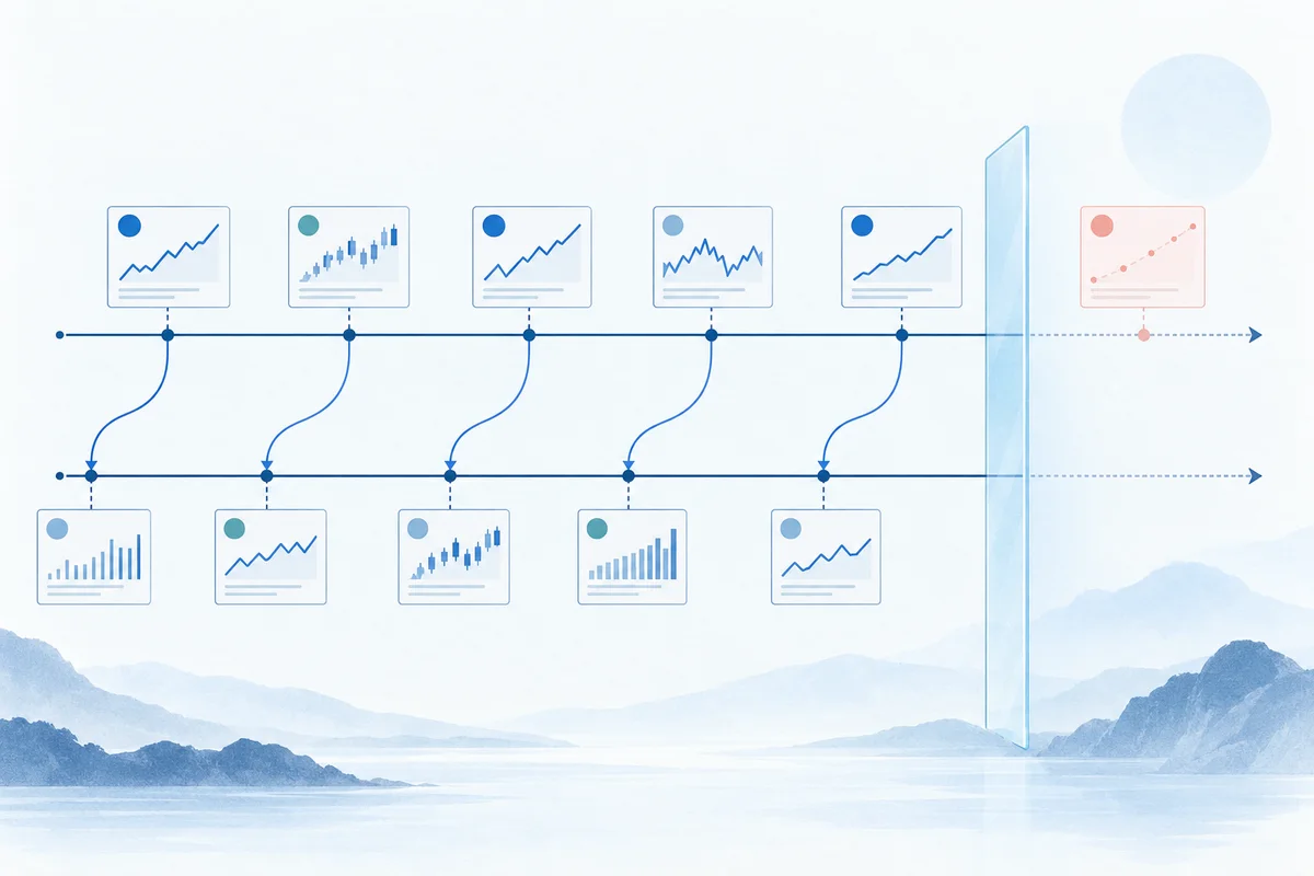
In quantitative finance, market information does not arrive on a synchronized global clock. A trading system consumes disparate data streams operating on entirely different frequencies and temporal mechanics:
- Regular OHLCV bars: Uniform sampling grids (e.g., 1-minute, 5-minute, or 1-hour candles) where a single row summarizes activity over a fixed duration.
- Asynchronous tick quotes: Millisecond-level National Best Bid and Offer (NBBO) updates that fire irregularly whenever market participants submit, cancel, or modify orders.
- Macroeconomic and fundamental announcements: Point-in-time event releases (such as US Nonfarm Payrolls, Consumer Price Index, or FOMC interest rate statements) published at discrete timestamps (e.g., 08:30:00.000 ET).
- Corporate earnings and SEC regulatory filings: Irregular filings (such as 10-Q and 8-K reports) disseminated outside normal trading hours with statutory publication delays.
When quantitative researchers prepare feature matrices for strategy evaluation, they must merge these asynchronous information feeds onto an execution timeline. Standard relational operations in pandas—such as pd.merge() or pd.concat()—fail catastrophically for this purpose:
- Inner joins (
how='inner'): Drop virtually every observation. High-frequency tick updates or macroeconomic releases almost never share the exact microsecond timestamp of an OHLCV bar close. - Outer joins (
how='outer'): Generate massive, sparse DataFrames populated by alternatingNaNvalues. To create continuous signals, researchers typically follow an outer join withdf.ffill(). However, if the sorting order is broken or if timestamp conventions between bar openings and bar closings are conflated, blind forward-filling silently leaks future price action backward in time.
Mathematically, let market history be modeled as a filtered probability space with filtration (F_t)_{t \ge 0}, representing the accumulated information set available up to time t. An admissible trading strategy generates an execution decision or signal A_t that must be strictly measurable with respect to F_t:
A_t \in F_t \quad \text{(Causal: evaluated strictly using information known at or before time } t \text{)}If your data alignment pipeline matches a price bar at time t with an event occurring at t + \Delta t (where \Delta t > 0), the strategy action becomes non-causal:
A_t \in F_{t + \Delta t} \quad \text{(Non-causal: evaluates future information before market publication)}This violation constitutes Lookahead Bias in Backtesting. It produces seductive backtest statistics—Sharpe ratios above 4.0, near-zero drawdowns, and 85%+ win rates—that collapse immediately when deployed into live capital execution.
To solve this temporal alignment problem without introducing lookahead bias, pandas provides pandas.merge_asof. When configured correctly, merge_asof performs an ordered, monotonic time-distance join that enforces strict causality across asynchronous data feeds.
Anatomy of pandas.merge_asof: Parameters and execution mechanics
The pandas.merge_asof function executes an "as-of" join between two DataFrames. Rather than searching for exact key equality, it matches each record in the left DataFrame with the nearest chronological record in the right DataFrame based on a continuous key (typically a datetime64[ns] timestamp).
Left DataFrame (Execution Timeline / Price Bars):
Time:      09:30:00        09:31:00        09:32:00        09:33:00
              │               │               │               │
Right Stream (Quotes / Macro Events):         │               │
Events:            09:30:42           09:31:15        09:32:05│
                      │                   │               │   │
                      ▼                   ▼               ▼   ▼
As-Of Match:     [No Prior]          [09:30:42]      [09:31:15]
                 (direction='backward' preserves strict temporal causality)
Both DataFrames must be sorted by the key column prior to calling merge_asof. The primary function signature and critical parameters are structured as follows:
pd.merge_asof(
    left,
    right,
    on=None,
    left_on=None,
    right_on=None,
    left_index=False,
    right_index=False,
    by=None,
    left_by=None,
    right_by=None,
    suffixes=("_x", "_y"),
    tolerance=None,
    allow_exact_matches=True,
    direction="backward",  # The pivotal parameter for causality
)
Parameter breakdown for quantitative developers
leftandright: The left DataFrame represents your primary driving clock (e.g., bar timestamps where execution decisions occur). The right DataFrame contains the secondary asynchronous stream (e.g., quotes, macro indicators, or alternative sentiment scores).on(orleft_on/right_on): The monotonic continuous key column. Both DataFrames must be sorted in ascending order along this column. If timestamps are unsorted, pandas raises an immediateValueError: left keys must be sorted.direction: Determines the temporal direction of the search window:'backward': Selects the most recent prior event (right_on <= left_on). This is the only causal direction safe for backtesting.'forward': Selects the next upcoming event (right_on >= left_on). This introduces explicit lookahead bias.'nearest': Selects the absolute closest event in time (min(|right_on - left_on|)). This silently peeks into future data whenever an upcoming event is closer than the preceding event.
allow_exact_matches: A boolean flag controlling boundary equality:True(default): Matchesright_on <= left_onunder'backward'.False: Enforces strict temporal precedenceright_on < left_on. This eliminates zero-millisecond execution miracles when publication and bar timestamps coincide.
tolerance: An integer, float, orpd.Timedeltadefining the maximum allowable distance between keys. If no event falls within the tolerance window, pandas populates the joined columns withNaN. This prevents ancient, stale market information from polluting current trading decisions.by(orleft_by/right_by): A categorical or identifier column (e.g.,ticker,symbol, orexchange) that requires exact string equality before performing the as-of time match.
Direction policies: Safe 'backward' vs hazardous 'nearest' and 'forward'
The choice of the direction argument is the single most critical decision when using merge_asof in a quantitative research workflow. Understanding the exact search mechanics of each policy prevents unintentional data leakage.
Timeline:              t_0 (Past)          t_bar (Decision)          t_1 (Future)
                            │                      │                      │
Events on Right Frame:      ● E_past               │                      ● E_future
Time Delta:                 |Δt_past| = 45s        │                      |Δt_future| = 15s
                                                   │
1. direction='backward':                           │
   Matches E_past <────────────────────────────────┘ (CAUSAL: E_past is known at t_bar)

2. direction='nearest':
   Matches E_future ──────────────────────────────────────────────────────> (FATAL LEAKAGE! 15s < 45s)

3. direction='forward':
   Matches E_future ──────────────────────────────────────────────────────> (FATAL LEAKAGE! Always looks ahead)
1. direction='backward' (The Causal Safe Harbor)
Under direction='backward', pandas searches backward along the timeline from the left record's timestamp. It retrieves the latest available record from the right DataFrame that satisfies:
\text{timestamp}_{\text{right}} \le \text{timestamp}_{\text{left}} \quad (\text{if allow\_exact\_matches=True})\text{timestamp}_{\text{right}} < \text{timestamp}_{\text{left}} \quad (\text{if allow\_exact\_matches=False})Because time moves strictly forward, an automated trading strategy evaluating an entry at 10:00:00 can only act upon market information that has already been recorded by the exchange or dissemination gateway at or before 10:00:00. Using direction='backward' guarantees that every feature in your model reflects historical reality.
2. direction='nearest' (The Silent Lookahead Trap)
Under direction='nearest', pandas computes the absolute temporal distance to both the preceding record and the subsequent record:
\text{argmin}_{i} \left| \text{timestamp}_{\text{right}, i} - \text{timestamp}_{\text{left}} \right|If an economic indicator is published at 08:30:00, and your left DataFrame contains 1-minute price bars ending at 08:29:00 and 08:30:00:
- For the
08:29:00bar, if the previous economic release was 30 days ago, the upcoming release at08:30:00is only 60 seconds away. direction='nearest'compares 30 days vs 60 seconds, selects the future08:30:00release, and attaches it to the08:29:00bar!
The model now holds economic announcement data 60 seconds before the announcement occurs. In a backtest, the strategy enters a position at the 08:29:00 price, effortlessly capturing the entire announcement volatility spike with zero drawdown.
3. direction='forward' (Unconditional Future Leakage)
Under direction='forward', pandas searches forward in time:
\text{timestamp}_{\text{right}} \ge \text{timestamp}_{\text{left}}This policy is useful for post-trade transaction cost analysis (e.g., evaluating price drift 5 minutes after an execution) or label creation in machine learning datasets. However, it must never be used to construct features or signals feeding a backtest.
Policy comparison matrix
| Policy Parameter | Temporal Search Condition | Causal Consistency | Lookahead Risk | Valid Quantitative Use Cases |
|---|---|---|---|---|
direction='backward' | t_right <= t_left | Strictly Causal | Zero (when timestamps are verified) | Signal generation, feature engineering, live bar alignment |
direction='nearest' | `min( | t_right - t_left | )` | Non-Causal |
direction='forward' | t_right >= t_left | Non-Causal | Guaranteed 100% Leakage | Target label creation (e.g., future returns), post-trade TCA |
Precision control: allow_exact_matches and temporal granularity
In high-frequency data engineering and event-driven backtesting, timestamp equality (t_left == t_right) introduces subtle edge cases that can compromise causal validity.
The zero-latency illusion
Consider a macroeconomic release published at exactly 08:30:00.000 UTC. If your trading bar represents a 1-minute period ending at 08:30:00.000 UTC, did your trading engine actually have access to that information at the moment the bar closed?
In reality:
- The Bureau of Labor Statistics or Federal Reserve releases the data feed.
- Financial news wires (Bloomberg, Refinitiv) and algorithmic aggregators ingest the payload.
- Network packets traverse fiber networks to your co-location facility or cloud instance (10–100 ms).
- Your internal parsing logic decodes the JSON, XML, or binary format and updates the feature matrix (5–50 ms).
If you merge with allow_exact_matches=True, pandas matches the 08:30:00.000 release directly with the 08:30:00.000 bar close. This assumes an instantaneous, zero-latency pipeline. If your backtest then assumes an order was executed at the 08:30:00.000 closing price, you have inadvertently traded on information that could not have physically arrived before the order book matched trades for that candle.
import pandas as pd

# Bar closing timestamps
bars = pd.DataFrame({
    "bar_time": pd.to_datetime([
        "2026-06-01 10:00:00.000",
        "2026-06-01 10:00:01.000",
        "2026-06-01 10:00:02.000",
    ]),
    "bar_close": [100.10, 100.25, 100.15],
}).sort_values("bar_time")

# Quote updates from market data feed
quotes = pd.DataFrame({
    "quote_time": pd.to_datetime([
        "2026-06-01 09:59:59.850",
        "2026-06-01 10:00:01.000",  # Exact collision with bar timestamp
        "2026-06-01 10:00:01.500",
    ]),
    "bid": [100.08, 100.24, 100.12],
    "ask": [100.12, 100.28, 100.16],
}).sort_values("quote_time")

# Case A: allow_exact_matches=True (Permissive)
aligned_permissive = pd.merge_asof(
    bars,
    quotes,
    left_on="bar_time",
    right_on="quote_time",
    direction="backward",
    allow_exact_matches=True,
)

# Case B: allow_exact_matches=False (Strictly prior)
aligned_strict = pd.merge_asof(
    bars,
    quotes,
    left_on="bar_time",
    right_on="quote_time",
    direction="backward",
    allow_exact_matches=False,
)
Inspecting the output at 10:00:01.000:
Permissive (allow_exact_matches=True):
                 bar_time  bar_close                quote_time     bid     ask
1 2026-06-01 10:00:01.000     100.25   2026-06-01 10:00:01.000  100.24  100.28

Strict (allow_exact_matches=False):
                 bar_time  bar_close                quote_time     bid     ask
1 2026-06-01 10:00:01.000     100.25   2026-06-01 09:59:59.850  100.08  100.12
By toggling allow_exact_matches=False, the model requires quote_time < bar_time. If a quote arrives simultaneously with the bar timestamp, the model refuses to assume it was readable in time to form that bar's closing decision.
Modeling realistic dissemination latency buffers
For external news feeds or macroeconomic reports, an even more robust engineering practice is to inject an explicit dissemination latency buffer directly into the right DataFrame before merging:
# Introduce a realistic 500ms network and parsing latency buffer
LATENCY_BUFFER = pd.Timedelta("500ms")
macro_data["available_at"] = macro_data["release_time"] + LATENCY_BUFFER

# Merge against the point-of-availability, NOT the official release timestamp
clean_features = pd.merge_asof(
    bars,
    macro_data,
    left_on="bar_time",
    right_on="available_at",
    direction="backward",
)
This guarantees that an economic figure released at 08:30:00.000 is only made visible to bars closing at or after 08:30:00.500.
Guarding against stale information: The tolerance parameter
While direction='backward' prevents looking forward into the future, it introduces a complementary risk: looking too far backward into the past.
Without bounds, merge_asof will search backward indefinitely until it finds a matching record. If an asset is halted, if an exchange connection drops, or if an illiquid security has not traded for four hours, an unbounded backward merge will pair the current candle with a four-hour-old quote.
09:30:00 Quote: Bid 100.00, Ask 100.05
    │
    ▼ [TRADING HALT / FEED DISCONNECTION FOR 3 HOURS]
    │
12:30:00 Bar Close: Unbounded merge_asof matches 09:30:00 quote!
Trading on stale quotes distorts portfolio accounting and generates phantom liquidity in your backtest. The solution is the tolerance parameter.
import pandas as pd

bars = pd.DataFrame({
    "timestamp": pd.to_datetime([
        "2026-06-01 10:00:00",
        "2026-06-01 10:01:00",
        "2026-06-01 10:05:00",  # 4-minute gap after market halt
    ]),
    "close": [150.0, 150.2, 148.5],
}).sort_values("timestamp")

quotes = pd.DataFrame({
    "timestamp": pd.to_datetime([
        "2026-06-01 09:59:58",
        "2026-06-01 10:00:55",
    ]),
    "bid": [149.95, 150.15],
    "ask": [150.05, 150.25],
}).sort_values("timestamp")

# Enforce a maximum allowable staleness window of 60 seconds
bounded_alignment = pd.merge_asof(
    bars,
    quotes,
    on="timestamp",
    direction="backward",
    tolerance=pd.Timedelta("60s"),
)
The resulting alignment demonstrates defensive data engineering:
            timestamp  close     bid     ask
0 2026-06-01 10:00:00  150.0  149.95  150.05  <- Matched 09:59:58 (2s old, within tolerance)
1 2026-06-01 10:01:00  150.2  150.15  150.25  <- Matched 10:00:55 (5s old, within tolerance)
2 2026-06-01 10:05:00  148.5     NaN     NaN  <- 4m > 60s tolerance -> Converted to NaN!
At row index 2, the most recent available quote was from 10:00:55 (4 minutes and 5 seconds earlier). Because this exceeds the 60-second tolerance, bid and ask are assigned NaN.
[!IMPORTANT] When
toleranceconverts stale values toNaN, do not blindly call.ffill(). ANaNin a preprocessed feature table indicates an illiquid halt or severed feed. Your trading logic should treatNaNas a trade suppression condition, vetoing new position entries until fresh market data resumes.
Multi-asset alignment: Grouping with the 'by' argument
Quantitative research rarely focuses on a single security in isolation. Multi-asset strategies must align quote streams, fundamental metrics, or order book depths across thousands of symbols simultaneously.
Naively iterating over tickers with Python for loops is slow, inefficient, and prone to indexing bugs. Instead, pandas.merge_asof provides the by argument (or left_by and right_by), which partitions both DataFrames by grouping keys before executing the as-of search.
The critical sorting requirement
When utilizing by, pandas enforces a strict prerequisite: the continuous on column must remain globally sorted in ascending order across the entire DataFrame.
import pandas as pd

# Multi-asset bar data
bars = pd.DataFrame({
    "timestamp": pd.to_datetime([
        "2026-06-01 09:30:00", "2026-06-01 09:30:00",
        "2026-06-01 09:31:00", "2026-06-01 09:31:00",
        "2026-06-01 09:32:00", "2026-06-01 09:32:00",
    ]),
    "symbol": ["AAPL", "MSFT", "AAPL", "MSFT", "AAPL", "MSFT"],
    "close": [180.10, 420.50, 180.40, 421.10, 180.25, 420.90],
}).sort_values("timestamp")

# Multi-asset quote stream with asynchronous arrival times
quotes = pd.DataFrame({
    "timestamp": pd.to_datetime([
        "2026-06-01 09:29:55",  # AAPL quote
        "2026-06-01 09:30:15",  # MSFT quote
        "2026-06-01 09:30:45",  # AAPL quote
        "2026-06-01 09:31:10",  # MSFT quote
    ]),
    "symbol": ["AAPL", "MSFT", "AAPL", "MSFT"],
    "bid": [180.05, 420.40, 180.35, 421.00],
    "ask": [180.15, 420.60, 180.45, 421.20],
}).sort_values("timestamp")

# Align quotes onto bars grouped by symbol with 60s tolerance
aligned_multi = pd.merge_asof(
    bars,
    quotes,
    on="timestamp",
    by="symbol",
    direction="backward",
    tolerance=pd.Timedelta("60s"),
)

print(aligned_multi)
Executing this code produces a partitioned alignment:
            timestamp symbol   close     bid     ask
0 2026-06-01 09:30:00   AAPL  180.10  180.05  180.15
1 2026-06-01 09:30:00   MSFT  420.50     NaN     NaN
2 2026-06-01 09:31:00   AAPL  180.40  180.35  180.45
3 2026-06-01 09:31:00   MSFT  421.10  420.40  420.60
4 2026-06-01 09:32:00   AAPL  180.25     NaN     NaN
5 2026-06-01 09:32:00   MSFT  420.90  421.00  421.20
Notice how merge_asof handles each security independently:
- Row 1 (
MSFTat09:30:00): The earliest recorded MSFT quote is at09:30:15. Because09:30:15is in the future relative to the bar timestamp, the backward join correctly yieldsNaN. MSFT is not contaminated by AAPL's09:29:55quote. - Row 3 (
MSFTat09:31:00): The MSFT quote from09:30:15is matched (45 seconds old, comfortably inside the 60s tolerance). - Row 4 (
AAPLat09:32:00): The most recent AAPL quote was recorded at09:30:45(75 seconds ago). Because 75s exceeds the 60s tolerance, the values are correctly set toNaN.
Concrete failure case: Macro announcement lookahead contamination
To see how a seemingly harmless alignment decision destroys strategy validity, consider an automated trading strategy operating on 1-minute bars around an important macroeconomic release (e.g., the Consumer Price Index published at 08:30:00 ET).
In this scenario:
- Prior to the release, the asset trades quietly between
100.00and100.20. - At
08:30:00, the CPI surprise prints at+2.5(a strongly bullish release). - During the
08:30:00to08:31:00window, market makers violently reprice the asset upward from100.20to103.00. - The strategy goes long whenever
cpi_surprise > 0.
Below is the complete Python reproduction demonstrating the flawed implementation versus the reconciled causal implementation:
import pandas as pd
import numpy as np

# 1. Primary execution timeline: 1-minute OHLC bars
bars = pd.DataFrame({
    "timestamp": pd.to_datetime([
        "2026-06-05 08:28:00",
        "2026-06-05 08:29:00",
        "2026-06-05 08:30:00",
        "2026-06-05 08:31:00",
        "2026-06-05 08:32:00",
        "2026-06-05 08:33:00",
    ]),
    "open":  [100.00, 100.10, 100.20, 103.00, 103.50, 103.40],
    "close": [100.10, 100.20, 103.00, 103.50, 103.40, 103.60],
}).sort_values("timestamp")

# 2. Macroeconomic release published at 08:30:00 ET
macro_events = pd.DataFrame({
    "release_time": pd.to_datetime(["2026-06-05 08:30:00"]),
    "cpi_surprise": [2.5],
}).sort_values("release_time")

# ==============================================================================
# FLAWED PIPELINE: Using direction='nearest' with a 90-second tolerance window
# ==============================================================================
flawed = pd.merge_asof(
    bars,
    macro_events,
    left_on="timestamp",
    right_on="release_time",
    direction="nearest",
    tolerance=pd.Timedelta("90s"),
)
flawed["signal"] = (flawed["cpi_surprise"] > 0).astype(float).fillna(0.0)

# ==============================================================================
# CAUSAL PIPELINE: Using direction='backward' with realistic 30s processing lag
# ==============================================================================
causal_events = macro_events.copy()
# Dissemination and parsing latency: data is physically actionable at 08:30:30
causal_events["available_time"] = causal_events["release_time"] + pd.Timedelta("30s")

causal = pd.merge_asof(
    bars,
    causal_events[["available_time", "cpi_surprise"]],
    left_on="timestamp",
    right_on="available_time",
    direction="backward",
)
causal["signal"] = (causal["cpi_surprise"] > 0).astype(float).fillna(0.0)

print("=== FLAWED ALIGNMENT (direction='nearest') ===")
print(flawed[["timestamp", "open", "close", "cpi_surprise", "signal"]])

print("\n=== CAUSAL ALIGNMENT (direction='backward' + 30s latency buffer) ===")
print(causal[["timestamp", "open", "close", "cpi_surprise", "signal"]])
Execution output analysis
=== FLAWED ALIGNMENT (direction='nearest') ===
            timestamp   open  close  cpi_surprise  signal
0 2026-06-05 08:28:00  100.0  100.1           NaN     0.0
1 2026-06-05 08:29:00  100.1  100.2           2.5     1.0  <- LOOKAHEAD!
2 2026-06-05 08:30:00  100.2  103.0           2.5     1.0
3 2026-06-05 08:31:00  103.0  103.5           2.5     1.0
4 2026-06-05 08:32:00  103.5  103.4           NaN     0.0
5 2026-06-05 08:33:00  103.4  103.6           NaN     0.0

=== CAUSAL ALIGNMENT (direction='backward' + 30s latency buffer) ===
            timestamp   open  close  cpi_surprise  signal
0 2026-06-05 08:28:00  100.0  100.1           NaN     0.0
1 2026-06-05 08:29:00  100.1  100.2           NaN     0.0
2 2026-06-05 08:30:00  100.2  103.0           NaN     0.0
3 2026-06-05 08:31:00  103.0  103.5           2.5     1.0  <- REALISTIC ENTRY
4 2026-06-05 08:32:00  103.5  103.4           2.5     1.0
5 2026-06-05 08:33:00  103.4  103.6           2.5     1.0
The catastrophic performance difference
Examine Row 1 (08:29:00) in the flawed alignment:
- The CPI announcement did not occur until
08:30:00. - However, because
direction='nearest'was applied with a 90-second tolerance,08:29:00was within 60 seconds of the future release. - The flawed backtest generates
signal = 1.0at08:29:00, entering a long position at100.10. - Over the next two bars, the asset reprices to
103.50. The backtester books a +3.40% profit (+3.4 points) with zero risk. The strategy appears to have supernatural market-timing abilities.
Now examine the causal alignment:
- The report was released at
08:30:00and became actionable after network/parsing delay at08:30:30. - The
08:30:00bar closed before08:30:30, socpi_surpriseremainedNaN(signal = 0.0). - The strategy receives the signal during the
08:31:00bar, entering long at the open of103.00. - Holding into
103.50yields a +0.49% profit (+0.50 points).
The +2.91% performance gap between the two models is purely synthetic: it is the exact value of the announcement repricing that occurred while the flawed model was holding a position it could not have legally entered in live trading.
Quantitative engineering checklist: 7 rules for causal data alignment
Before piping preprocessed DataFrames into simulation frameworks like OpenBacktesting, run your feature pipelines through this 7-point audit checklist.
                    ┌────────────────────────────────────────────────────────┐
                    │       CAUSAL DATA ALIGNMENT VERIFICATION AUDIT         │
                    └────────────────────────────────────────────────────────┘
                                                 │
          ┌──────────────────┬───────────────────┼───────────────────┬──────────────────┐
          ▼                  ▼                   ▼                   ▼                  ▼
    1. Monotonic Sort  2. Timezone Parity  3. Boundary Meaning 4. Latency Buffer  5. Direction
    - is_monotonic_inc - Explicit UTC      - Open vs Close     - Network/Parsing  - 'backward' ONLY
    - Strict ascending - No naive mixing   - Avoid t=t leaks   - Buffer > 0 ms    - Never 'nearest'
          │                                                                             │
          └──────────────────────────────┬──────────────────────────────────────────────┘
                                         ▼
                          ┌─────────────────────────────┐
                          │    6. Tolerance Boundaries  │  - Set staleness cap
                          │    7. Defensive NaN Vetoes  │  - NaN = Veto trade
                          └─────────────────────────────┘
1. Monotonic ascending sorting verification
Pandas will fail or produce silent errors if timestamps are not strictly ascending. Validate both DataFrames prior to merging:
assert df_bars["timestamp"].is_monotonic_increasing, "Bars are not monotonically sorted!"
assert df_events["timestamp"].is_monotonic_increasing, "Events are not monotonically sorted!"
2. Timezone parity enforcement
Ensure both series share identical timezone specifications. Merging a timezone-naive datetime64[ns] against a timezone-aware datetime64[ns, UTC] triggers a TypeError: Cannot compare tz-naive and tz-aware timestamps. Standardize all sources to UTC:
df_bars["timestamp"] = pd.to_datetime(df_bars["timestamp"], utc=True)
df_events["timestamp"] = pd.to_datetime(df_events["timestamp"], utc=True)
3. Clear bar boundary semantics
Document whether your bar timestamps indicate the start or the end of the candle. If a bar labeled 09:30:00 represents the interval [09:30:00, 09:31:00), merging an event from 09:30:45 onto 09:30:00 via backward matching is an error because the event occurred after the bar open. Always align asynchronous information to the timestamp corresponding to the moment an order decision is evaluated.
4. Mandatory dissemination latency buffers
Never assume zero-latency data transport. For corporate earnings, economic numbers, or analyst consensus revisions, add an explicit conservative transmission buffer:
df_events["available_time"] = df_events["published_time"] + pd.Timedelta(seconds=10)5. Strict backward direction constraint
Enforce direction='backward' for all feature alignment tasks. Prohibit direction='nearest' across all production backtesting repositories through code review or automated linter rules.
6. Bounded tolerance windows
Always define an explicit tolerance parameter tailored to the frequency of the underlying asset class. If a tick feed is interrupted, tolerance guarantees that obsolete prices are converted to NaN rather than forward-filled indefinitely.
7. Defensive null handling and signal vetoes
Post-merge NaN values must not be blindly smoothed or forward-filled. Treat missing or stale features as an automatic trading veto:
# Suppress signals whenever required features are missing or stale
valid_data_mask = aligned_df[["feature_a", "feature_b"]].notna().all(axis=1)
trading_signal = raw_signal.where(valid_data_mask, 0.0)
Integrating clean alignments into OpenBacktesting
Once your feature matrices and price series are causally aligned via pandas.merge_asof, they can be passed directly into an execution simulation engine.
OpenBacktesting (0.2.1) is an independent Python backtesting engine built for Python >=3.12,<3.15 that specializes in single-asset historical OHLCV bar-by-bar research. By decoupling feature engineering from execution simulation, OpenBacktesting allows you to maintain strict causality:
- Pre-backtest data hygiene: Clean your historical OHLCV series and merge asynchronous event features using
pandas.merge_asof(direction='backward'). - Deterministic bar-by-bar evaluation: OpenBacktesting steps through your preprocessed data bar by bar, ensuring that signals evaluated at bar
tclose can only generate orders executed at bart+1open or through explicit limit orders. - Inspectable trial persistence: All orders, executions, and equity trajectories are recorded to SQLite, allowing you to visually inspect trades in the local Studio UI and verify that no trades occurred prior to historical event publication timestamps.
By combining pandas.merge_asof with disciplined causality checks, quantitative researchers can eliminate lookahead bias at the data engineering layer before running a single simulation trial.