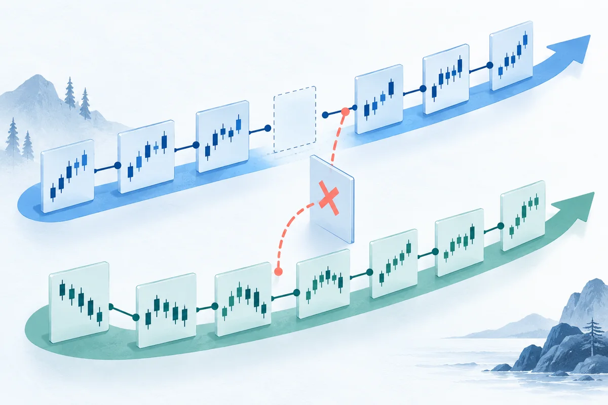
The return engineering pipeline: Vectorized percentage changes in Pandas
In algorithmic trading and quantitative portfolio research, financial time series almost never enter alpha models as raw price quotes. Raw prices are non-stationary, exhibit unit roots, and vary across arbitrary order-of-magnitude scales between different assets. To normalize asset price movements into stationary sequences suitable for cross-sectional ranking, factor analysis, risk attribution, and Sharpe ratio evaluation, quantitative engineers transform raw closing prices into return sequences.
In the Python data science ecosystem, pandas.DataFrame.pct_change() and pandas.Series.pct_change() serve as the standard vectorized primitives for computing discrete percentage changes across successive observations. Under the hood, for a discrete price series P evaluated across index steps t with lag parameter periods=k (where default k=1), the method computes the discrete simple relative return:
R_t = (P_t - P_{t-k}) / P_{t-k} = (P_t / P_{t-k}) - 1flowchart TD
A["Raw Historical Market Data\n(OHLCV Bars / Ticker Panels)"] --> B["Data Hygiene & Alignment\n• Chronological Sorting: sort_values(['ticker', 'date'])\n• Timestamp De-duplication & Resampling"]
B --> C{"DataFrame Structure?"}
C -->|"Single-Asset Time Series"| D["Direct Vectorized Calculation\ns.pct_change(periods=1)"]
C -->|"Multi-Asset Long Panel"| E["Grouped Boundary Isolation\ndf.groupby('ticker')['close'].pct_change()"]
C -->|"Multi-Asset Wide Matrix"| F["Cross-Sectional Column Vectorization\ndf.pivot(index='date', columns='ticker').pct_change()"]
D --> G["Defensive Validation Layer\n• NaN Cascade Audit (P_t vs P_t-1 missingness)\n• Scale Verification (Decimal 0.05 vs Percentage 5.0)\n• Boundary Isolation: nth(0).isna().all()\n• Physical Solvency Guard: R_t > -1.0"]
E --> G
F --> G
G --> H["Validated Strategy Alpha Pipeline\n• Momentum & Mean-Reversion Signals\n• Bar-by-Bar Simulation / OpenBacktesting"]While calculating df['Close'].pct_change() appears deceptively simple on a pristine, single-ticker tutorial dataset, executing it in production research pipelines exposes severe mathematical and structural hazards:
- Fractional Decimal vs. Percentage Mismatch: Treating a fractional output of
0.05as5.0—or vice versa—causes catastrophic compounding errors in downstream wealth accumulation curves and introduces 100x variance distortions in volatility metrics. - Missing Value Invalidation Cascades: Missing bars do not simply produce a single
NaN. A single missing price point invalidates two consecutive returns unless handled explicitly. - The
fill_methodDeprecation Traps: Historical versions of Pandas silently forward-filled missing prices by default (fill_method='pad'), generating artificial zero-return observations that suppressed realized volatility. Modern Pandas (version 2.1 and later) deprecates and restricts this parameter, necessitating explicit imputations. - Cross-Asset Boundary Contamination: Applying
df['Close'].pct_change()across an unsorted or stacked multi-asset panel calculates the return between the closing price of Ticker A and the opening bar of Ticker B, injecting artificial multi-hundred-percent outliers into momentum signals and factor rankings.
Engineering robust quantitative signals requires mastering the exact behavior of pct_change(), understanding its numerical conventions, and implementing automated boundary assertions before feeding returns into backtest engines.
Decimal fractions vs percentages: The mathematical convention
A frequent point of confusion among quantitative developers transitioning from spreadsheet tools or broker terminals to Python is the unit convention returned by pandas.Series.pct_change().
The dimensionless ratio convention
pandas.Series.pct_change() returns a decimal fraction (a dimensionless ratio), not a percentage representation scaled from 0 to 100:
- An asset advancing from $100.00 to $105.00 yields
0.05, not5.0. - An asset dropping from $100.00 to $90.00 yields
-0.10, not-10.0. - An asset suffering a total loss to $0.00 yields
-1.00, not-100.0.
import pandas as pd

prices = pd.Series([100.0, 105.0, 94.5], name="Close")
returns = prices.pct_change()

print("Raw Prices:")
print(prices)
print("\npct_change() Output (Decimal Fraction):")
print(returns)Raw Prices:
0 100.0
1 105.0
2 94.5
Name: Close, dtype: float64
pct_change() Output (Decimal Fraction):
0 NaN
1 0.05
2 -0.10
Name: Close, dtype: float64The catastrophic compounding bug
When quantitative researchers compute cumulative returns or track an equity curve, they compound periodic returns using the identity:
V_T = V_0 * \prod_{t=1}^T (1 + R_t)In vectorized Python code, this is implemented via:
equity_curve = initial_capital * (1 + returns).cumprod()If your pipeline erroneously multiplies returns by 100—or ingests data from an external provider that pre-multiplied returns by 100—evaluating (1 + returns) transforms a standard 5% gain (0.05) into (1 + 5.0) = 6.0. Over a single step, the equity curve registers a 500% gain instead of a 5% gain. Over ten bars, the portfolio compounds to astronomical, nonsensical values:
import numpy as np
import pandas as pd

# True decimal returns: 1% daily gain over 5 days
r_decimal = pd.Series([0.01] * 5)

# Erroneously scaled percentage returns: 1.0 representing 1%
r_percent = pd.Series([1.0] * 5)

capital = 10_000.0

correct_wealth = capital * (1 + r_decimal).cumprod()
corrupted_wealth = capital * (1 + r_percent).cumprod()

comparison = pd.DataFrame({
    "Step": range(1, 6),
    "Decimal (Correct)": correct_wealth,
    "Percentage Scaled (Corrupted)": corrupted_wealth
})
print(comparison.to_string(index=False)) Step Decimal (Correct) Percentage Scaled (Corrupted)
1 10100.00 20000.00
2 10201.00 40000.00
3 10303.01 80000.00
4 10406.04 160000.00
5 10510.10 320000.00Volatility and Sharpe ratio distortion
The same scale error devastates risk metrics. The sample standard deviation \sigma of returns scaled as 5.0 is exactly 100 times larger than \sigma computed on 0.05. Because the Sharpe ratio divides excess return by volatility:
Sharpe = (E[R] - R_f) / \sigma(R)If E[R] and \sigma(R) are consistently scaled by 100, the scalar cancels out in a zero-risk-free regime. However, if an engineer mixes an unscaled annual risk-free rate (such as 0.04 for 4%) with percentage-scaled daily returns (mean = 0.08, std = 1.2), subtracting 0.04 from 0.08 generates an erroneous excess return calculation that invalidates the strategy's Sharpe score.
Simple returns vs. continuous log returns
While pct_change() calculates simple arithmetic returns, many stochastic models and risk frameworks operate on continuous log returns:
Simple Return:  R_t = (P_t - P_{t-1}) / P_{t-1} = (P_t / P_{t-1}) - 1
Log Return: r_t = ln(P_t / P_{t-1}) = ln(1 + R_t)┌─────────────────────────────────────────────────────────────────────────────┐
│ SIMPLE VS. LOGARITHMIC RETURN METRICS │
├──────────────────────┬──────────────────────────┬───────────────────────────┤
│ Characteristic │ Simple Return (R_t) │ Log Return (r_t) │
├──────────────────────┼──────────────────────────┼───────────────────────────┤
│ Pandas Formulation │ df['Close'].pct_change() │ np.log(df['Close']/ │
│ │ │ df['Close'].shift())│
│ Time Aggregation │ Compounded: \prod(1+R_t) │ Additive: \sum(r_t) │
│ Cross-Asset Aggregate│ Linear: \sum(w_i * R_i) │ Non-linear approximation │
│ Lower Bound │ -1.0 (-100%) │ -\infty │
│ Upper Bound │ +\infty │ +\infty │
│ Economic Meaning │ Realized cash flow ratio │ Continuously compounded │
└──────────────────────┴──────────────────────────┴───────────────────────────┘When building multi-asset portfolio accounting systems, simple returns must be used for cross-sectional portfolio aggregation, because the return of a portfolio is the linear weighted sum of the simple returns of its constituent assets:
R_{portfolio, t} = \sum_{i=1}^N w_{i, t} * R_{i, t}The weighted sum of logarithmic returns does not equal the portfolio log return due to Jensen's Inequality. However, when aggregating returns across consecutive time intervals for a single asset, log returns provide computational convenience because multi-period returns collapse to simple summation.
Missing value dynamics: The fill_method deprecation and NaN cascades
One of the most consequential breaking changes in modern Pandas quantitative workflows centers around missing value handling in pct_change().
Historical context: The silent padding flaw (Pandas < 2.1)
In versions of Pandas prior to 2.1.0, Series.pct_change() defaulted to fill_method='pad'. When a price series encountered missing data (NaN or None), Pandas silently forward-filled the prior price observation before calculating the percentage change.
Consider a price series where a trading halt, delayed open, or network interruption causes missing quotes:
Raw Prices: [100.0, NaN, 105.0]Under Pandas < 2.1 with default padding:
NaNat index 1 was forward-filled to100.0.- The price series became
[100.0, 100.0, 105.0]. - Returns computed:
[NaN, 0.0, 0.05].
This behavior was deeply problematic for financial research. A missing bar was transformed into an artificial zero-return bar (0.0). In systematic strategies, injecting artificial zero returns:
- Artificially deflates realized return variance and suppresses volatility estimates.
- Confuses market closures with genuine flat market sessions.
- In intraday market-making models, masks quotes that failed to execute due to exchange outages.
Modern Pandas (2.1+ and 3.0+): Mandatory explicit imputation
Recognizing the hazard of implicit data imputation, the Pandas core team deprecated fill_method in Pandas 2.1.0. In modern releases (Pandas 2.2+ and Pandas 3.0+), passing fill_method raises an explicit error:
import pandas as pd

series = pd.Series([100.0, None, 105.0])

try:
    series.pct_change(fill_method="pad")
except ValueError as exc:
print(f"Raised Expected Error: {exc}")Raised Expected Error: fill_method must be None; got fill_method='pad'.The deprecation requires quantitative engineers to make an explicit domain decision: how should missing market data be resolved before calculating returns?
The double-NaN cascade phenomenon
When pct_change() executes on a series containing missing values without prior imputation, it triggers a double-NaN cascade:
import pandas as pd

series = pd.Series([100.0, None, 105.0, 110.25], index=pd.date_range("2026-01-01", periods=4))
returns = series.pct_change()

print("Price Series:")
print(series)
print("\nDirect pct_change():")
print(returns)Price Series:
2026-01-01 100.00
2026-01-02 NaN
2026-01-03 105.00
2026-01-04 110.25
Freq: D, dtype: float64
Direct pct_change():
2026-01-01 NaN
2026-01-02 NaN
2026-01-03 NaN
2026-01-04 0.05
Freq: D, dtype: float64Notice what occurred:
2026-01-01: First observation has no predecessor, yieldingNaN.2026-01-02: Price isNaN. Formula evaluates(NaN - 100.0) / 100.0 = NaN.2026-01-03: Price is105.0, but predecessor isNaN. Formula evaluates(105.0 - NaN) / NaN = NaN.2026-01-04: Price is110.25, predecessor is105.0. Formula evaluates(110.25 - 105.0) / 105.0 = 0.05.
A single missing price bar on 2026-01-02 destroyed two consecutive return observations. If a dataset has isolated missing values scattered across 5% of its rows, a naive pct_change() call can wipe out up to 10% of your strategy's valid return history.
Strategic solutions for missing values
Quantitative engineers generally adopt one of three explicit strategies depending on market structure:
import pandas as pd

prices = pd.Series([100.0, None, 105.0, 110.25])

# Strategy A: Explicit forward-fill (Assumes last traded price persists)
# Creates a 0.0 return at index 1, computes return from 100.0 to 105.0 at index 2
ret_ffill = prices.ffill().pct_change()

# Strategy B: Drop missing bars prior to return calculation
# Compares 105.0 directly to 100.0, ignoring time elapsed
ret_dropped = prices.dropna().pct_change()

# Strategy C: Raw calculation followed by explicit forward masking
ret_raw = prices.pct_change()

print("Strategy A (Explicit ffill):\n", ret_ffill)
print("\nStrategy B (Dropna first):\n", ret_dropped)
print("\nStrategy C (Raw with cascade):\n", ret_raw)Strategy A (Explicit ffill):
0 NaN
1 0.00
2 0.05
3 0.05
dtype: float64
Strategy B (Dropna first):
0 NaN
2 0.05
3 0.05
dtype: float64
Strategy C (Raw with cascade):
0 NaN
1 NaN
2 NaN
3 0.05
dtype: float64For rigorous backtesting, Strategy A is appropriate if an illiquid instrument's position mark-to-market assumes the asset remains valued at the last traded price. However, when evaluating momentum factors, Strategy B is superior because a missing day should not be counted as zero-drift volatility.
The silent killer: Cross-asset boundary contamination
The single most destructive error in quantitative data preparation occurs when applying pct_change() to a multi-asset panel DataFrame stored in long (stacked) format.
The panel data stitch mechanism
In modern quantitative architectures, asset prices are frequently stored in tabular long panels where multiple tickers are stacked vertically:
┌────────────────────────────────────────────────────────┐
│              STACKED PANEL DATA STRUCTURE              │
├───────┬────────────┬────────┬──────────────────────────┤
│ Index │ Ticker     │ Date   │ Close                    │
├───────┼────────────┼────────┼──────────────────────────┤
│ 0     │ AAPL       │ Day 1  │ 180.00                   │
│ 1     │ AAPL       │ Day 2  │ 182.00                   │
│ 2     │ AAPL       │ Day 3  │ 185.00  <-- AAPL End     │
│ 3     │ MSFT       │ Day 1  │ 420.00  <-- MSFT Start   │
│ 4     │ MSFT       │ Day 2  │ 425.00                   │
│ 5     │ MSFT       │ Day 3  │ 430.00                   │
└───────┴────────────┴────────┴──────────────────────────┘
If an engineer executes df['return'] = df['Close'].pct_change(), Pandas operates strictly along the positional index. At row index 3, Pandas computes:
R_3 = (Close_3 - Close_2) / Close_2
    = (420.00 - 185.00) / 185.00
    = +1.27027 (+127.03%)
This single computation stitches Apple's final close to Microsoft's opening close. It manufactures an artificial, synthetic +127% single-day return that never occurred in the financial markets.
import pandas as pd

# Demonstrating cross-asset boundary contamination
panel = pd.DataFrame({
    "ticker": ["AAPL", "AAPL", "AAPL", "MSFT", "MSFT", "MSFT"],
    "date": pd.to_datetime(["2026-01-05", "2026-01-06", "2026-01-07"] * 2),
    "close": [180.00, 182.00, 185.00, 420.00, 425.00, 430.00]
})

# NAIVE APPROACH: Corrupts cross-asset boundary
panel["naive_return"] = panel["close"].pct_change()

# CORRECT APPROACH: Grouped return calculation
panel["grouped_return"] = panel.groupby("ticker")["close"].pct_change()

print(panel[["ticker", "date", "close", "naive_return", "grouped_return"]]) ticker date close naive_return grouped_return
0 AAPL 2026-01-05 180.0 NaN NaN
1 AAPL 2026-01-06 182.0 0.011111 0.011111
2 AAPL 2026-01-07 185.0 0.016484 0.016484
3 MSFT 2026-01-05 420.0 1.270270 NaN
4 MSFT 2026-01-06 425.0 0.011905 0.011905
5 MSFT 2026-01-07 430.0 0.011765 0.011765Downstream damage of boundary contamination
In a universe of 500 equities evaluated across ten years of daily data:
- Top-Quintile Momentum Contamination: A cross-sectional momentum strategy ranking assets by past returns will select MSFT immediately following the transition boundary, because its fake +127% return catapults it to the top decile. The strategy enters a long position based entirely on an engineering artifact.
- Mean-Reversion Disasters: A short-term mean-reversion strategy seeking extreme overbought conditions will aggressively short MSFT at row 3, predicting a collapse from an artificial spike.
- Z-Score Normalization Collapse: Cross-sectional standardization
(R - mean) / stdcalculated across the universe on2026-01-05will have its mean and standard deviation blown out by the +1.27 outlier, compressing the z-scores of all 499 genuine assets toward zero. - Machine Learning Feature Distortion: When training neural networks or gradient-boosted trees on lagged return features, boundary artifacts become influential outliers, causing tree splits that memorize ticker transition points rather than true market patterns.
The unsorted DataFrame hazard
Even within a single ticker, pct_change() calculates differences between adjacent rows in their current DataFrame order. If market data ingested from an external database or Parquet store is not strictly sorted chronologically:
import pandas as pd

unordered = pd.DataFrame({
    "date": pd.to_datetime(["2026-01-07", "2026-01-05", "2026-01-06"]),
    "close": [185.0, 180.0, 182.0]
})

unordered["corrupted_return"] = unordered["close"].pct_change()

# Proper sorting
ordered = unordered.sort_values("date").reset_index(drop=True)
ordered["correct_return"] = ordered["close"].pct_change()

print("Unordered pct_change (Corrupted temporal order):")
print(unordered)
print("\nSorted pct_change (Valid temporal sequence):")
print(ordered)Unordered pct_change (Corrupted temporal order):
date close corrupted_return
0 2026-01-07 185.0 NaN
1 2026-01-05 180.0 -0.027027
2 2026-01-06 182.0 0.011111
Sorted pct_change (Valid temporal sequence):
date close correct_return
0 2026-01-05 180.0 NaN
1 2026-01-06 182.0 0.011111
2 2026-01-07 185.0 0.016484In the unsorted DataFrame, row 1 computes a return from Jan 7 to Jan 5 (-2.70%), computing a backwards-in-time synthetic delta.
Production data patterns: Long panels vs wide matrices
To prevent cross-asset boundary leakage and temporal corruption, quantitative systems rely on two standardized data architectures.
Pattern 1: Long panel with explicit group transformation
When maintaining long-format data, always chain sort_values() before applying groupby().pct_change():
import pandas as pd

def compute_panel_returns(df: pd.DataFrame, ticker_col: str = "ticker", date_col: str = "date", price_col: str = "close") -> pd.DataFrame:
    """Sorts long panel data chronologically by asset and computes isolated returns."""
    df_sorted = df.sort_values(by=[ticker_col, date_col]).copy()
    df_sorted["return"] = df_sorted.groupby(ticker_col)[price_col].pct_change()
    return df_sorted
This guarantees:
- Rows are strictly ascending by date within each ticker.
- The return calculation resets to
NaNat the first observation of every distinct ticker. - No cross-asset contamination occurs.
Pattern 2: Wide format matrix pivoting
For multi-asset portfolio rebalancing, factor investing, and risk modeling, transforming long panels into wide price matrices where columns represent tickers and the index represents timestamps eliminates boundary leakage by architectural design:
import pandas as pd

panel = pd.DataFrame({
    "ticker": ["AAPL", "AAPL", "AAPL", "MSFT", "MSFT", "MSFT"],
    "date": pd.to_datetime(["2026-01-05", "2026-01-06", "2026-01-07"] * 2),
    "close": [180.00, 182.00, 185.00, 420.00, 425.00, 430.00]
})

# Pivot to wide format: Index=Date, Columns=Ticker
prices_wide = panel.pivot(index="date", columns="ticker", values="close")

# Vectorized pct_change across columns independently (down axis=0)
returns_wide = prices_wide.pct_change()

print("Wide Price Matrix:")
print(prices_wide)
print("\nWide Return Matrix (Zero cross-asset leakage):")
print(returns_wide)Wide Price Matrix:
ticker AAPL MSFT
date
2026-01-05 180.0 420.0
2026-01-06 182.0 425.0
2026-01-07 185.0 430.0
Wide Return Matrix (Zero cross-asset leakage):
ticker AAPL MSFT
date
2026-01-05 NaN NaN
2026-01-06 0.011111 0.011905
2026-01-07 0.016484 0.011765Because prices_wide.pct_change() operates vertically along the date axis independently for each column, boundary contamination is mathematically impossible. Both assets correctly record NaN on the first trading date.
Defensive data engineering: Unit tests and validation assertions
Production data engineering requires active validation rather than passive assumption. Before any return series enters a backtest simulation or signal engine, it must pass automated defensive assertions.
The subtle Pandas trap: groupby.first() drops NaNs!
When validating that every ticker's initial bar contains a NaN return, many developers write:
# WARNING: SUBTLE BUG IN UNIT TEST ASSERTION
assert df.groupby('ticker')['return'].first().isna().all()
In Pandas, GroupBy.first() skips null values by default (dropna=True). If row 0 of a ticker group is NaN and row 1 is 0.011, groupby('ticker')['return'].first() will return 0.011! The assertion will fail on valid, boundary-isolated data!
To correctly inspect the true first row of each group including null values, use .nth(0):
# CORRECT DEFENSIVE CHECK
assert df.groupby('ticker')['return'].nth(0).isna().all()
Comprehensive panel validation suite
The following production script implements a complete defensive validation pipeline. It checks boundary isolation, physical solvency bounds, decimal scaling sanity, and temporal monotonicity.
import pandas as pd
import numpy as np

def audit_return_series(
    df: pd.DataFrame,
    ticker_col: str = "ticker",
    date_col: str = "date",
    return_col: str = "return"
) -> dict[str, bool]:
    """Executes production data hygiene checks on computed return sequences."""
    audit_results = {}

    # Check 1: Boundary Isolation
    # The first bar of EVERY ticker group MUST be NaN
    first_bars = df.groupby(ticker_col)[return_col].nth(0)
    audit_results["boundary_isolation_passed"] = bool(first_bars.isna().all())

    # Check 2: Physical Solvency Bound
    # In standard long-only cash equity markets, returns cannot drop below -100% (-1.0)
    valid_returns = df[return_col].dropna()
    audit_results["solvency_bound_passed"] = bool((valid_returns > -1.0).all())

    # Check 3: Scale Sanity Check (Fractional Decimal vs Percentage)
    # A daily return > 1.0 represents a +100% gain in a single bar.
    # While possible during extreme short squeezes, if > 1% of bars exceed 1.0,
    # the series was almost certainly scaled as a percentage (0-100) instead of decimal (0-1).
    extreme_outliers = (valid_returns.abs() > 1.0).mean()
    audit_results["scale_decimal_passed"] = bool(extreme_outliers < 0.01)

    # Check 4: Temporal Monotonicity
    # Timestamps within each ticker must be strictly ascending
    is_monotonic = df.groupby(ticker_col)[date_col].apply(
        lambda s: s.is_monotonic_increasing
    ).all()
    audit_results["monotonic_time_passed"] = bool(is_monotonic)

    return audit_results


# Unit Test Execution
if __name__ == "__main__":
    # Test Dataset with intentional multi-asset structure
    test_data = pd.DataFrame({
        "ticker": ["AAPL", "AAPL", "AAPL", "MSFT", "MSFT", "MSFT"],
        "date": pd.to_datetime(["2026-01-05", "2026-01-06", "2026-01-07"] * 2),
        "close": [180.0, 182.0, 185.0, 420.0, 425.0, 430.0]
    })

    # 1. Compute Naive Returns (Corrupted Boundary)
    test_data["naive_return"] = test_data["close"].pct_change()

    # 2. Compute Safe Returns (Isolated Boundary)
    test_data["safe_return"] = test_data.groupby("ticker")["close"].pct_change()

    naive_audit = audit_return_series(test_data, return_col="naive_return")
    safe_audit = audit_return_series(test_data, return_col="safe_return")

    print("--- NAIVE RETURN AUDIT (Expect Failure) ---")
    for check, passed in naive_audit.items():
        print(f"  {check}: {'PASS' if passed else 'FAIL'}")

    print("\n--- SAFE RETURN AUDIT (Expect Pass) ---")
    for check, passed in safe_audit.items():
print(f" {check}: {'PASS' if passed else 'FAIL'}")--- NAIVE RETURN AUDIT (Expect Failure) ---
boundary_isolation_passed: FAIL
solvency_bound_passed: PASS
scale_decimal_passed: FAIL
monotonic_time_passed: PASS
--- SAFE RETURN AUDIT (Expect Pass) ---
boundary_isolation_passed: PASS
solvency_bound_passed: PASS
scale_decimal_passed: PASS
monotonic_time_passed: PASSRunning this audit suite flags the naive return series immediately:
boundary_isolation_passed: FAILbecause MSFT's first observation contains the +1.27 stitch return rather thanNaN.scale_decimal_passed: FAILbecause the boundary stitch created an artificial +127% jump that triggered the scale anomaly detector.
Architecture alignment: Single-asset backtesting in OpenBacktesting
While vectorized Pandas operations like pct_change() provide rapid exploratory signal screening, transitioning from signal generation to institutional backtesting requires an execution engine that eliminates lookahead and boundary leakage by design.
Why event-driven and bar-by-bar engines eliminate boundary leakage
In vectorized backtesting, strategies operate on entire columns of data simultaneously (df['signal'] * df['return']). A single indexing error, missing shift (shift(1)), or un-grouped pct_change() leaks future prices or cross-asset data across the entire backtest timeline.
In contrast, OpenBacktesting (version 0.2.1, targeting Python >=3.12,<3.15) is an independent Python backtesting engine built specifically for single-asset historical OHLCV bar-by-bar research:
- Sequential Bar-by-Bar Processing: OpenBacktesting iterates through historical OHLCV bars sequentially. The strategy receives bar
tat timet, with zero programmatic access to bart+1. Boundary leakage between distinct tickers is architecturally impossible because each backtest trial executes on an isolated, single-asset price feed. - Inspectable Orders and Fills: Rather than assuming executions occur at theoretical percentage changes, OpenBacktesting logs discrete orders, matching fills against actual bar prices (Open, High, Low, Close) with configurable slippage and transaction fee models.
- SQLite Trial Persistence: Every backtest trial, order log, and equity curve is stored in a local SQLite database, allowing quants to inspect individual trade executions in the local Studio UI and verify that calculated PnL corresponds to exact fills rather than corrupted vectorized returns.
- Data Contract Enforcement: Before passing market data to OpenBacktesting, running validation checks such as those outlined in our Backtesting Data Checklist ensures that data feeds are sorted, free of unhandled missing gaps, and correctly aligned with market calendar sessions.
Vectorized return engineering checklist
Before deploying any feature engineering or quantitative alpha model relying on pandas pct_change, verify your pipeline against this operational checklist:
┌─────────────────────────────────────────────────────────────────────────────┐
│                 VECTORIZED RETURN DATA ENGINEERING AUDIT                    │
├─────────────────────┬────────────────────────────┬──────────────────────────┤
│ Potential Trap      │ Vulnerable Pattern         │ Defensive Solution       │
├─────────────────────┼────────────────────────────┼──────────────────────────┤
│ Scale Confusion     │ Treating 0.05 as 5.0       │ Assert abs(r) < 1.0 for  │
│                     │ in wealth compounding      │ 99%+ of liquid bars      │
│                     │                            │                          │
│ Missing Bar Cascade │ Direct pct_change() over   │ Explicit ffill() or      │
│                     │ un-imputed missing quotes  │ dropna() with time-gap   │
│                     │                            │ calendar tracking        │
│                     │                            │                          │
│ fill_method Crash   │ s.pct_change(fill_method=  │ Remove fill_method param │
│                     │ 'pad') in Pandas 2.1+/3.0+ │ (use s.ffill().pct_      │
│                     │                            │ change() explicitly)     │
│                     │                            │                          │
│ Panel Stitch Leak   │ df['Close'].pct_change()   │ df.groupby('ticker')     │
│                     │ on long-form panel         │   ['Close'].pct_change() │
│                     │                            │                          │
│ Temporal Jumps      │ pct_change() on unsorted   │ df.sort_values(          │
│                     │ timestamp index            │   ['ticker', 'date'])    │
│                     │                            │                          │
│ Groupby Test Flaw   │ groupby().first().isna()   │ groupby().nth(0).isna()  │
│                     │ (.first() drops NaNs!)     │ (preserves group head)   │
└─────────────────────┴────────────────────────────┴──────────────────────────┘
Actionable engineering rules
- Never apply
pct_change()to raw long-form panels: Always enforcedf.groupby('ticker')['close'].pct_change(), or pivot your data into a wide matrix (df.pivot(index='date', columns='ticker', values='close')) where cross-asset stitching is structurally impossible. - Sort before transforming: Always enforce
df.sort_values(by=['ticker', 'date'])prior to calling difference or return operations. - Handle missing values explicitly: With
fill_methoddeprecated in modern Pandas, never rely on default padding. Explicitly choose between forward-filling (ffill()) to maintain regular time grids or dropping bars (dropna()) to analyze active quote changes. - Guard your test assertions: When writing unit tests with
pytest, remember thatGroupBy.first()drops missing values by default. Usedf.groupby('ticker')['return'].nth(0).isna().all()to verify that every ticker begins with an uncomputedNaNreturn. - Enforce cash solvency: Ensure all calculated daily returns satisfy
R_t > -1.0(-100%) for non-leveraged assets. Any return below-1.0signals either corrupted data or inverted price quotes. - Decouple signal research from execution: Use vectorized Pandas returns for initial hypothesis testing, but execute final strategy evaluations in an isolated, bar-by-bar engine like OpenBacktesting to protect your capital from lookahead bias and cross-asset contamination.