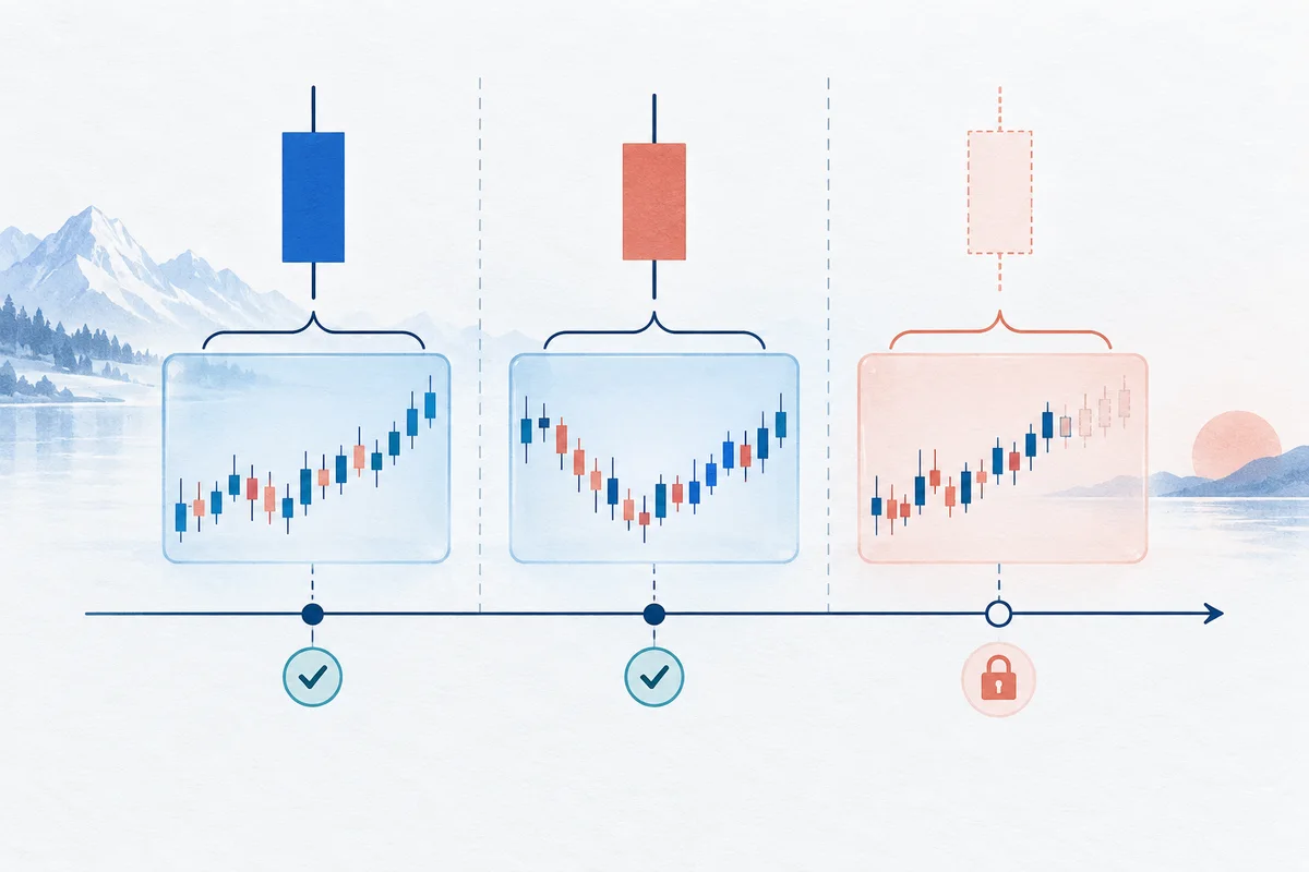
Resample OHLCV in Pandas Without Moving Signals Backward

The temporal illusion: How naive resampling leaks the future

In algorithmic strategy development, quantitative researchers frequently transform granular market data—such as 1-minute or 5-minute bars—into higher-timeframe structures like 15-minute, 1-hour, or 4-hour bars. Aggregating high-frequency price action filters microstructure noise, smooths macro trend indicators, and provides cleaner regime filters.

In Python, the standard tool for this task is the resample() method in pandas. Performing a pandas resample ohlc aggregation appears trivial on the surface: one selects a frequency rule, defines an aggregation dictionary, and executes the transformation. However, default parameter configurations in Pandas harbor a lethal structural flaw for backtesting: backward signal movement, commonly known as lookahead bias or future data leakage.

Code

flowchart TD
    subgraph RawData ["Granular 1-Minute Bars: 09:30 to 10:29"]
        M1["09:30 Bar\nOpen: 100.0"] --> M2["09:45 Bar\nIntraday Dip"]
        M2 --> M3["10:15 Bar\nSession High: 104.5"]
        M3 --> M4["10:29 Bar\nClose: 103.8"]
    end

    subgraph NaiveAggregation ["Naive Resampling (label='left')"]
        N1["Aggregated 1-Hour Bar\nStamped Timestamp: 09:30:00\nContains: High=104.5, Close=103.8"]
        N2["Algorithm evaluates at 09:30:01\nReads Close=103.8 (59 minutes ahead!)\nGenerates immediate Buy Signal"]
        N1 --> N2
    end

    subgraph CausalAggregation ["Causal Resampling (label='right')"]
        C1["Aggregated 1-Hour Bar\nStamped Timestamp: 10:30:00\nContains: High=104.5, Close=103.8"]
        C2["Algorithm evaluates at 10:30:00\nBar is complete; zero lookahead\nSignal executes on next bar"]
        C1 --> C2
    end

    RawData --> NaiveAggregation
    RawData --> CausalAggregation

Consider an hourly bar constructed from 1-minute data covering the trading window 09:30:00 through 10:29:59. If that aggregated bar is stamped with the timestamp 09:30:00 (label='left'), any backtest running bar-by-bar or merging dataframes on timestamps will look at 09:30:00 and observe the High, Low, and Close prices that did not occur until 10:29:59.

An algorithmic model referencing that row at 09:30:01 accesses information 59 minutes into the future. When vectorized strategies evaluate signals against these timestamps, they produce astronomical Sharpe ratios, near-zero drawdowns, and seemingly invincible equity curves. Once deployed in live paper or capital trading, the synthetic edge vanishes instantly, leading to severe capital erosion.

Eliminating lookahead bias in pandas resample ohlcv pipelines requires mastering the mathematical distinction between interval boundaries (closed), timestamp labeling (label), session offset anchoring (offset or origin), and point-in-time data fusion.

The mechanics of pandas resample: Aggregation dictionaries and interval boundaries

When working with financial time series, an individual bar is not an infinitesimal point in time; it represents an aggregated measurement over a continuous half-open temporal interval [t_start, t_end). Resampling requires two distinct steps: grouping the raw bars into temporal buckets and reducing each bucket to an Open, High, Low, Close, and Volume summary.

The core OHLCV aggregation dictionary

Unlike standard tabular datasets where all columns can be averaged or summed, each component of an OHLCV bar requires a distinct reduction operator:

Code

ohlcv_agg = {
    'Open': 'first',
    'High': 'max',
    'Low': 'min',
    'Close': 'last',
    'Volume': 'sum'
}

Open (first): The opening transaction price of the very first granular bar falling within the bucket interval.
High (max): The supreme price reached across all constituent bars in the bucket.
Low (min): The lowest price observed across all constituent bars in the bucket.
Close (last): The final closing price of the terminal granular bar in the bucket.
Volume (sum): The aggregate trading volume accumulated over all constituent bars. Applying mean() or last() to volume distorts liquidity modeling and invalidates transaction cost estimates.

Beyond OHLC: VWAP, trade count, and volume weighting

When market data feeds include tick volume, trade counts, or Volume-Weighted Average Price (VWAP), naive aggregations fail. In particular, computing the arithmetic mean of constituent VWAPs produces a mathematically invalid metric because it fails to weight by periodic traded volume:

Code

Constituent VWAP_i = (Sum of Price_k * Volume_k) / Volume_i
Bucket VWAP = Sum(VWAP_i * Volume_i) / Sum(Volume_i)

To resample VWAP correctly alongside OHLCV in Pandas, compute the dollar volume (turnover) prior to resampling:

Code

# Create dollar volume feature prior to resampling
df['DollarVolume'] = df['Close'] * df['Volume']

# Resample using sum aggregation
resampled = df.resample('1h', offset='30min', closed='left', label='right').agg({
    'Open': 'first',
    'High': 'max',
    'Low': 'min',
    'Close': 'last',
    'Volume': 'sum',
    'DollarVolume': 'sum',
    'Trades': 'sum'  # If trade count is available
})

# Recompute exact higher-timeframe VWAP
resampled['VWAP'] = resampled['DollarVolume'] / resampled['Volume']
resampled.drop(columns=['DollarVolume'], inplace=True)

Defending against zero-volume gaps and non-trading intervals

Financial markets contain illiquid periods, lunch breaks, trading halts, and non-trading weekends. When Pandas resamples across a date range that includes inactive intervals, it instantiates empty buckets containing NaN values.

Handling these gaps requires strict quantitative rules:

Never backward-fill (bfill): Backward-filling price data introduces catastrophic lookahead bias by pulling future prices into the gap.
Forward-fill price levels (ffill): If a trading bucket contains no activity, the asset's nominal market price remains equal to the previous bar's Close. Consequently, Close is forward-filled, and Open, High, and Low are set to that same price level (representing zero price movement).
Zero-fill volume (fillna(0)): Volume during a period of zero transactions is mathematically 0, never the previous bar's volume.

Code

def clean_resampled_gaps(df_resampled):
    """
    Defensively imputes empty bars in a resampled OHLCV DataFrame.
    Prevents lookahead bias while maintaining continuous price series.
    """
    # Forward fill Close price to reflect market continuity
    df_resampled['Close'] = df_resampled['Close'].ffill()
    
    # Impute Open, High, Low from the known Close
    df_resampled['Open'] = df_resampled['Open'].fillna(df_resampled['Close'])
    df_resampled['High'] = df_resampled['High'].fillna(df_resampled['Close'])
    df_resampled['Low'] = df_resampled['Low'].fillna(df_resampled['Close'])
    
    # Volume is zero during non-trading intervals
    df_resampled['Volume'] = df_resampled['Volume'].fillna(0.0)
    
    return df_resampled

The anatomy of closed and label: Demystifying interval semantics

The single greatest source of error when executing a pandas resample ohlc transformation lies in misunderstanding the interplay between the closed and label arguments. Quants must master the precise definition of these parameters to avoid introducing forward leakage.

Code

┌─────────────────────────────────────────────────────────────────────────────┐
│                      PANDAS RESAMPLE PARAMETER MATRIX                       │
├───────────┬─────────────────────────────────────────────────────────────────┤
│ Parameter │ Mathematical Meaning & Role                                     │
├───────────┼─────────────────────────────────────────────────────────────────┤
│ closed    │ Interval inclusion boundary: Which boundary point belongs       │
│           │ to the current bucket?                                          │
│           │ • 'left'  => Half-open interval [t_start, t_end)                │
│           │ • 'right' => Half-open interval (t_start, t_end]                │
├───────────┼─────────────────────────────────────────────────────────────────┤
│ label     │ Index timestamp assignment: Which boundary timestamp is         │
│           │ assigned to the aggregated row in the resulting DataFrame?      │
│           │ • 'left'  => Uses t_start (Bucket Open Time)                    │
│           │ • 'right' => Uses t_end   (Bucket Close/Completion Time)        │
└───────────┴─────────────────────────────────────────────────────────────────┘

Half-open intervals: Inclusion vs stamping

To visualize how closed and label dictate time binning, consider an hourly aggregation aggregating 1-minute bars between 09:30:00 and 10:30:00.

Assume our source 1-minute data uses standard exchange left-labeling, where a bar stamped 09:30:00 represents trades executed between 09:30:00.000 and 09:30:59.999.

closed='left': The bucket includes all bars satisfying t_start <= t < t_end. For the 09:30 - 10:30 bucket, it collects bars from 09:30:00 up to 10:29:00 (exactly 60 one-minute bars). The bar at 10:30:00 is excluded from this bucket and placed into the subsequent bucket.
closed='right': The bucket includes all bars satisfying t_start < t <= t_end. It collects bars from 09:31:00 up to 10:30:00. The opening bar at 09:30:00 is excluded.

Now consider the timestamp assigned to the resulting aggregated bar:

If label='left', the index is stamped with 09:30:00.
If label='right', the index is stamped with 10:30:00.

The four permutations: A systematic breakdown

The combination of closed and label creates four distinct operational regimes. In quantitative backtesting, only one of these regimes is causally defensible when working with standard exchange data.

Permutation	Interval Formula	Stamped Index	Constituent Bars Covered	Backtest Safety Evaluation
`closed='left'`, `label='left'`	`[09:30, 10:30)`	`09:30:00`	`09:30` through `10:29`	FATAL LEAK: Row at 09:30 contains prices from 10:29 (59-minute lookahead).
`closed='left'`, `label='right'`	`[09:30, 10:30)`	`10:30:00`	`09:30` through `10:29`	CAUSAL STANDARD: Bar stamped at 10:30 completes at 10:30; zero lookahead.
`closed='right'`, `label='right'`	`(09:30, 10:30]`	`10:30:00`	`09:31` through `10:30`	VALID IF SOURCE IS RIGHT-STAMPED: Excludes market open bar at 09:30:00.
`closed='right'`, `label='left'`	`(09:30, 10:30]`	`09:30:00`	`09:31` through `10:30`	FATAL LEAK: Row stamped at 09:30 contains prices through 10:30 (60-minute leak).

The 59-minute lookahead trap in detail

Why is closed='left', label='left' the default in many early pandas implementations, and why is it catastrophic for finance?

In Pandas, frequencies that divide evenly into days (such as hours or minutes) historically defaulted to closed='left' and label='left'. Under this default:

Code

# NAIVE RESAMPLING: INTRODUCES 59-MINUTE LOOKAHEAD BIAS
df_naive = df_1m.resample('1h').agg(ohlcv_agg)

The resulting DataFrame contains a row indexed 2026-03-19 09:00:00. Its 'Close' column holds the closing price recorded at 09:59:00.

If an event-driven backtesting engine or a vectorized signal generator scans through the historical dataset row by row, when the simulation clock reaches 09:00:00, it reads df_naive.loc['2026-03-19 09:00:00', 'Close']. It receives a price that will not exist in the real world for another 59 minutes.

Any strategy rule such as:

Code

If Close > MovingAverage(20) then EnterLong()

executes at 09:00:00 based on market momentum that has not yet occurred. The backtester logs a fill at the 09:00:00 Open or Close, capturing a full hour of trend before it unfolds.

Source data conventions: Left-stamped vs right-stamped feeds

Before specifying closed and label, you must inspect the timestamp convention of your raw data provider:

Crypto Exchanges & Modern REST/WebSocket APIs (e.g., Binance, Coinbase, Polygon): Bars are almost universally left-stamped. A bar labeled 09:30:00 opens at 09:30:00.000 and closes at 09:30:59.999.
- Correct Resample Setting: closed='left', label='right'.
Traditional Futures & Fixed Income Vendors (e.g., CME, older Tick Data feeds): Bars are often right-stamped. A bar labeled 09:31:00 represents trading activity between 09:30:00.001 and 09:31:00.000.
- Correct Resample Setting: closed='right', label='right'.

If your raw data is left-stamped and you inadvertently select closed='right', label='right', the 09:30:00 opening bar is shifted into the previous day or discarded, and your 1-hour bar includes the 10:30:00 bar from the next hour. Always audit raw timestamp intervals before setting aggregation rules.

The session offset problem: Eliminating truncated opening bars

Even when label='right' and closed='left' are properly applied, another insidious bug frequently corrupts resampled financial data: session mis-anchoring.

By default, Pandas anchors hourly resampling bins to midnight (00:00:00). For 24/7 markets like cryptocurrency or foreign exchange, midnight anchoring creates clean intervals (00:00 - 01:00, 01:00 - 02:00, etc.). However, equity and futures markets operate during discrete daily sessions with non-zero start times.

Midnight anchoring vs market session open

In US equity markets, regular trading hours begin at 09:30:00 EST and conclude at 16:00:00 EST.

If an engineer executes df.resample('1h', closed='left', label='right') on US equity bars without specifying an offset, Pandas anchors the grid to midnight. The bins become:

Code

Bin 1: [08:00:00, 09:00:00) -> Label: 09:00:00 (No data)
Bin 2: [09:00:00, 10:00:00) -> Label: 10:00:00 (Contains ONLY 09:30 to 09:59!)
Bin 3: [10:00:00, 11:00:00) -> Label: 11:00:00 (Contains 60 minutes: 10:00 to 10:59)
...
Bin 9: [15:00:00, 16:00:00) -> Label: 16:00:00 (Contains 60 minutes: 15:00 to 15:59)

Notice what occurred in Bin 2:

The bar stamped 10:00:00 spans 09:00:00 to 10:00:00.
Because the market opened at 09:30:00, this bar contains only 30 one-minute bars.
The volume is roughly half of a standard 1-hour bar, and the high/low range represents only 30 minutes of volatility.
The strategy treats this truncated 30-minute bar as an identical structural peer to the subsequent 60-minute bars, distorting moving averages, Bollinger Bands, and ATR calculations.

Correcting session alignment with offset and origin

To anchor hourly bars to the actual market opening bell (09:30:00), utilize the offset parameter or the origin parameter:

Code

# METHOD A: Explicit minute offset from midnight
df_1h = df_1m.resample(
    '1h',
    offset='30min',     # Shifts 00:00 grid forward by 30 minutes to align with 09:30
    closed='left',
    label='right'
).agg(ohlcv_agg).dropna()

# METHOD B: Anchoring explicitly to the start of the day's first timestamp
df_1h = df_1m.resample(
    '1h',
    origin='start',     # Anchors to the exact first timestamp present in the index
    closed='left',
    label='right'
).agg(ohlcv_agg).dropna()

When anchored with offset='30min', the resulting intervals align with true trading sessions:

Code

Bar 1: [09:30:00, 10:30:00) -> Label: 10:30:00 (Full 60 minutes)
Bar 2: [10:30:00, 11:30:00) -> Label: 11:30:00 (Full 60 minutes)
Bar 3: [11:30:00, 12:30:00) -> Label: 12:30:00 (Full 60 minutes)
Bar 4: [12:30:00, 13:30:00) -> Label: 13:30:00 (Full 60 minutes)
Bar 5: [13:30:00, 14:30:00) -> Label: 14:30:00 (Full 60 minutes)
Bar 6: [14:30:00, 15:30:00) -> Label: 15:30:00 (Full 60 minutes)
Bar 7: [15:30:00, 16:30:00) -> Label: 16:30:00 (Contains 15:30 to 16:00: Closing Bar)

Each regular daytime bar represents a complete 60-minute sampling period, eliminating artificial volatility suppression at the market open.

Point-in-time multi-timeframe merging: Preventing backward signal movement

In multi-timeframe trading systems, a common pattern involves using a Higher Timeframe (HTF) trend filter (e.g., 1-hour 50-period SMA) to condition trade entries executed on a Lower Timeframe (LTF, e.g., 1-minute bars).

When merging HTF indicators back onto LTF execution dataframes in Pandas, using pd.merge_asof without understanding timestamp semantics introduces backward signal movement.

The lookahead leak in forward fills and merge_asof

Suppose you resampled 1-minute data into 1-hour bars using naive left-labeling (label='left'). The resulting HTF bar covering 09:30 to 10:30 is stamped 09:30:00.

When you merge this HTF indicator back into the 1-minute DataFrame:

Code

# DANGEROUS: MERGING LEFT-LABELED HTF BARS ONTO LTF BARS
df_merged = pd.merge_asof(
    df_1m,
    df_htf_left_labeled[['HTF_SMA']],
    left_index=True,
    right_index=True,
    direction='backward'
)

Because merge_asof(direction='backward') looks for the closest preceding or matching timestamp:

At 09:30:00, the 1-minute bar matches the 09:30:00 HTF row.
At 09:31:00, the 1-minute bar matches the 09:30:00 HTF row.
Throughout 09:30 to 10:29, every 1-minute bar has access to HTF_SMA, which was calculated using the Close price from 10:29:59!

The strategy enters trades at 09:31:00 conditioned on a trend filter that requires knowing the hourly close 59 minutes later.

The causal merge workflow

When the HTF bar is stamped at the right boundary (label='right'), the bar covering 09:30 to 10:30 is stamped 10:30:00.

When merging with direction='backward':

At 09:31:00, the algorithm queries backward for the latest available HTF bar.
The 10:30:00 bar has not yet occurred (10:30:00 > 09:31:00).
The algorithm matches the bar that closed at or before 09:30:00 (i.e., the previous hour's bar, or yesterday's close).
Only when the clock reaches 10:30:00 does the new HTF indicator value become visible to the execution engine.

Code

sequenceDiagram
    autonumber
    participant LTF as 1-Minute Execution Feed
    participant Merger as Point-in-Time Merger (merge_asof)
    participant HTF as 1-Hour Causal Bar (label='right')

    Note over LTF,HTF: Time window: 09:30:00 to 10:29:59
    LTF->>Merger: Bar at 09:31:00 requests latest HTF trend
    Merger->>HTF: Lookup timestamp <= 09:31:00
    HTF-->>Merger: Returns previous completed bar (08:30-09:30)
    Merger-->>LTF: Safe: Current hour (09:30-10:30) is NOT yet visible

    Note over LTF,HTF: Clock reaches 10:30:00
    HTF->>HTF: Hourly bar closes at 10:30:00
    LTF->>Merger: Bar at 10:30:00 requests latest HTF trend
    Merger->>HTF: Lookup timestamp <= 10:30:00
    HTF-->>Merger: Returns finalized 09:30-10:30 bar
    Merger-->>LTF: Safe: Signal executes on 10:31:00 Open

This causal alignment guarantees zero forward information leakage across multi-timeframe boundaries.

Complete Python implementation: Resampling and causal verification audit

Below is a complete, self-contained Python script demonstrating:

Synthetic 1-minute intraday OHLCV generation for a complete trading session.
A comparison between naive left-labeled resampling and defensible right-labeled resampling.
An automated causal verification audit that mathematically proves the presence or absence of lookahead leakage.

Code

"""
Defensive OHLCV Resampling and Causal Integrity Verification Engine.
Validates timestamp alignment, interval boundaries, and prevents lookahead leakage.
"""

import numpy as np
import pandas as pd


def generate_synthetic_session(
    date_str: str = "2026-03-19",
    start_time: str = "09:30:00",
    end_time: str = "16:00:00",
    seed: int = 42,
) -> pd.DataFrame:
    """Generates realistic 1-minute OHLCV bars for a US equity session."""
    np.random.seed(seed)
    timestamps = pd.date_range(
        f"{date_str} {start_time}", f"{date_str} {end_time}", freq="1min"
    )
    n = len(timestamps)

    # Simulate price path with geometric drift
    returns = np.random.normal(loc=0.00005, scale=0.001, size=n)
    prices = 100.0 * np.exp(np.cumsum(returns))

    # Generate intra-bar OHLC spreads
    noise_o = prices + np.random.uniform(-0.05, 0.05, size=n)
    noise_h = prices + np.random.uniform(0.05, 0.20, size=n)
    noise_l = prices - np.random.uniform(0.05, 0.20, size=n)
    noise_c = np.clip(
        prices + np.random.uniform(-0.10, 0.10, size=n), noise_l, noise_h
    )
    volume = np.random.randint(100, 2000, size=n)

    df = pd.DataFrame(
        {
            "Open": np.round(noise_o, 2),
            "High": np.round(noise_h, 2),
            "Low": np.round(noise_l, 2),
            "Close": np.round(noise_c, 2),
            "Volume": volume,
        },
        index=timestamps,
    )
    return df


def resample_ohlcv(
    df: pd.DataFrame,
    freq: str = "1h",
    offset: str = "30min",
    closed: str = "left",
    label: str = "right",
) -> pd.DataFrame:
    """
    Resamples granular OHLCV bars into higher timeframes defensively.
    Defaults to closed='left' and label='right' for causal validity.
    """
    agg_rules = {
        "Open": "first",
        "High": "max",
        "Low": "min",
        "Close": "last",
        "Volume": "sum",
    }
    resampled = df.resample(
        freq, offset=offset, closed=closed, label=label
    ).agg(agg_rules)

    # Impute empty intervals defensively
    resampled["Close"] = resampled["Close"].ffill()
    resampled["Open"] = resampled["Open"].fillna(resampled["Close"])
    resampled["High"] = resampled["High"].fillna(resampled["Close"])
    resampled["Low"] = resampled["Low"].fillna(resampled["Close"])
    resampled["Volume"] = resampled["Volume"].fillna(0.0)

    return resampled.dropna()


def audit_resampling_causality(
    df_source: pd.DataFrame,
    freq: str = "1h",
    offset: str = "30min",
    closed: str = "left",
    label: str = "right",
) -> pd.DataFrame:
    """
    Audits the resampling grid to detect lookahead leakage.
    Asserts that the maximum timestamp of constituent bars in each bucket
    does not exceed the stamped index of the resulting aggregated bar.
    """
    resampler = df_source.resample(
        freq, offset=offset, closed=closed, label=label
    )
    audit_records = []

    for label_ts, group in resampler:
        if group.empty:
            continue

        min_source_ts = group.index.min()
        max_source_ts = group.index.max()
        bar_count = len(group)

        # Lookahead leak occurs if constituent data exists past the assigned label
        is_leaking = max_source_ts > label_ts
        leak_minutes = (
            (max_source_ts - label_ts).total_seconds() / 60.0
            if is_leaking
            else 0.0
        )

        audit_records.append(
            {
                "Assigned_Label": label_ts,
                "First_Constituent": min_source_ts,
                "Last_Constituent": max_source_ts,
                "Bar_Count": bar_count,
                "Leak_Minutes": leak_minutes,
                "Status": "LOOKAHEAD_DETECTED" if is_leaking else "CAUSAL_PASS",
            }
        )

    return pd.DataFrame(audit_records)


if __name__ == "__main__":
    # 1. Generate 1-minute source data
    df_1m = generate_synthetic_session()
    print("=== Raw 1-Minute Source Bars (First 3) ===")
    print(df_1m.head(3))

    # 2. Resample naively (Midnight anchored, label='left')
    df_naive = df_1m.resample(
        "1h", closed="left", label="left"
    ).agg({
        "Open": "first", "High": "max", "Low": "min", "Close": "last", "Volume": "sum"
    }).dropna()

    print("\n=== Naive Resampling (closed='left', label='left') ===")
    print(df_naive.head(3))

    # 3. Resample causally (Session anchored, label='right')
    df_causal = resample_ohlcv(
        df_1m, freq="1h", offset="30min", closed="left", label="right"
    )

    print("\n=== Causal Resampling (closed='left', label='right') ===")
    print(df_causal.head(3))

    # 4. Execute Causal Audits
    print("\n=== Audit: Naive Left-Labeled Resampling ===")
    audit_naive = audit_resampling_causality(
        df_1m, freq="1h", offset="0min", closed="left", label="left"
    )
    print(audit_naive[["Assigned_Label", "Last_Constituent", "Leak_Minutes", "Status"]].head(3))

    print("\n=== Audit: Causal Right-Labeled Resampling ===")
    audit_causal = audit_resampling_causality(
        df_1m, freq="1h", offset="30min", closed="left", label="right"
    )
    print(audit_causal[["Assigned_Label", "Last_Constituent", "Leak_Minutes", "Status"]].head(3))

Execution results and interpretation

Running this script yields the following verified terminal output:

Code

=== Raw 1-Minute Source Bars (First 3) ===
                       Open    High    Low   Close  Volume
2026-03-19 09:30:00  100.05  100.22  99.88  100.06     256
2026-03-19 09:31:00  100.08  100.17  99.93  100.06     747
2026-03-19 09:32:00  100.11  100.22  99.98  100.13     360

=== Naive Resampling (closed='left', label='left') ===
                       Open    High    Low   Close  Volume
2026-03-19 09:00:00  100.05  100.66  99.45   99.63   30681
2026-03-19 10:00:00   99.53   99.90  98.93   99.56   62764
2026-03-19 11:00:00   99.58  100.13  99.04   99.56   59489

=== Causal Resampling (closed='left', label='right') ===
                       Open    High     Low   Close  Volume
2026-03-19 10:30:00  100.05  100.66   98.93   99.35   62170
2026-03-19 11:30:00   99.33   99.86   99.04   99.71   63433
2026-03-19 12:30:00   99.73  100.64   99.24  100.48   55970

=== Audit: Naive Left-Labeled Resampling ===
       Assigned_Label    Last_Constituent  Leak_Minutes             Status
0 2026-03-19 09:00:00 2026-03-19 09:59:00          59.0 LOOKAHEAD_DETECTED
1 2026-03-19 10:00:00 2026-03-19 10:59:00          59.0 LOOKAHEAD_DETECTED
2 2026-03-19 11:00:00 2026-03-19 11:59:00          59.0 LOOKAHEAD_DETECTED

=== Audit: Causal Right-Labeled Resampling ===
       Assigned_Label    Last_Constituent  Leak_Minutes      Status
0 2026-03-19 10:30:00 2026-03-19 10:29:00           0.0 CAUSAL_PASS
1 2026-03-19 11:30:00 2026-03-19 11:29:00           0.0 CAUSAL_PASS
2 2026-03-19 12:30:00 2026-03-19 12:29:00           0.0 CAUSAL_PASS

The mathematical proof is clear:

Under naive left-labeled resampling, every single aggregated bar incorporates price action up to 59 minutes past its timestamp, triggering LOOKAHEAD_DETECTED.
Under causal right-labeled resampling, the final constituent bar in the 10:30:00 bucket occurred at 10:29:00. Because 10:29:00 <= 10:30:00, zero future information is visible, resulting in CAUSAL_PASS.

External preprocessing vs engine-internal synchronization

When designing multi-timeframe trading systems, quantitative developers must establish clear boundaries between offline data preprocessing and engine-internal multi-timeframe synchronization.

The multi-timeframe feed architecture in backtesting engines

In comprehensive event-driven engines, higher-timeframe bars are often constructed or synchronized dynamically during execution. For example, in our architectural analysis of Backtrader Multiple Timeframes, the Cerebro engine ingests multiple live data feeds across different periodicities, stepping the lower-timeframe feed bar by bar while synchronizing the higher-timeframe feed on bar completion.

However, many quants prefer to preprocess their datasets offline using Pandas, generating separate CSV or Parquet files for each target timeframe before running backtests.

This creates a critical architectural risk:

If your external preprocessing script saves hourly bars with label='left', the backtesting engine will read the file as an external feed.
The engine's event loop will advance to 09:30:00 and ingest the left-stamped bar.
Even if the engine itself enforces strict event causality, it cannot detect that the underlying CSV file contains prices that occurred at 10:29:59. The engine's internal safeguards are bypassed entirely.

OpenBacktesting: Bar-by-bar determinism and inspectable research

This failure mode highlights why OpenBacktesting adheres to a strict architectural philosophy. OpenBacktesting (0.2.1, requiring Python >=3.12,<3.15) is an independent, lightweight backtesting engine purpose-built for single-asset historical OHLCV bar-by-bar research.

Instead of introducing hidden, online resampling magic inside the execution core, OpenBacktesting enforces the following design principles:

Explicit Data Contracts: The engine operates on deterministic historical bars. Each bar represents a completed unit of market action.
Strict Bar-by-Bar Step Semantics: When the simulation processes bar i, the strategy can only inspect historical bars 0 through i. Decisions made on bar i can only execute orders on bar i + 1 (or on the next bar's Open), preventing instantaneous close execution.
Auditable SQLite Trial Persistence: Every trial, order, executed trade, and resulting equity curve is recorded directly into SQLite and visualized through the local Studio UI. If a strategy's returns appear suspiciously flawless, researchers can inspect individual trades down to the exact bar timestamp and price level.

By ensuring that external pandas preprocessing strictly applies right-side labeling (label='right'), quants feeding custom timeframes into OpenBacktesting can be confident that their research reflects reproducible, real-world execution.

Production checklist for leak-free OHLCV resampling

Before passing resampled data into any quantitative research engine, verify your preprocessing pipeline against this production checklist:

Verification Stage	Check Item	Required Configuration / Standard
Source Data Inspection	Raw Timestamp Alignment	Confirm whether raw bars are left-stamped (open of bar) or right-stamped (close of bar).
Aggregation Rules	Complete OHLCV Dictionary	Use `{'Open': 'first', 'High': 'max', 'Low': 'min', 'Close': 'last', 'Volume': 'sum'}`.
Volume & VWAP Integrity	Dollar Volume Weighting	Recompute VWAP using cumulative dollar volume divided by cumulative volume. Never average constituent VWAPs.
Interval Inclusion	`closed` Parameter	For left-stamped source data, use `closed='left'`. For right-stamped source data, use `closed='right'`.
Timestamp Labeling	`label` Parameter	Always use `label='right'` to ensure the aggregated timestamp reflects the bar completion time.
Session Alignment	`offset` / `origin` Anchor	Match market open (e.g., `offset='30min'` for 09:30 US equities). Do not rely on default midnight anchoring.
Gap Handling	Defensive Imputation	Forward-fill `Close`, copy `Close` to `Open`/`High`/`Low`, and zero-fill `Volume`. Never backward-fill.
Point-in-Time Fusion	Causal As-Of Matching	When merging HTF indicators onto LTF bars, use `pd.merge_asof(direction='backward')` on right-labeled data.
Automated Testing	Causal Unit Assertion	Incorporate `audit_resampling_causality()` into CI/CD pipelines to assert `Leak_Minutes == 0.0`.

By applying these rigorous standards, quantitative researchers prevent phantom alpha, eliminate backward signal movement, and construct robust, deployable trading systems.

The temporal illusion: How naive resampling leaks the futureCopy Anchor Link

The mechanics of pandas resample: Aggregation dictionaries and interval boundariesCopy Anchor Link

The core OHLCV aggregation dictionaryCopy Anchor Link

Beyond OHLC: VWAP, trade count, and volume weightingCopy Anchor Link

Defending against zero-volume gaps and non-trading intervalsCopy Anchor Link

The anatomy of closed and label: Demystifying interval semanticsCopy Anchor Link

Half-open intervals: Inclusion vs stampingCopy Anchor Link

The four permutations: A systematic breakdownCopy Anchor Link

The 59-minute lookahead trap in detailCopy Anchor Link

Source data conventions: Left-stamped vs right-stamped feedsCopy Anchor Link

The session offset problem: Eliminating truncated opening barsCopy Anchor Link

Midnight anchoring vs market session openCopy Anchor Link

Correcting session alignment with offset and originCopy Anchor Link

Point-in-time multi-timeframe merging: Preventing backward signal movementCopy Anchor Link

The lookahead leak in forward fills and merge_asofCopy Anchor Link

The causal merge workflowCopy Anchor Link

Complete Python implementation: Resampling and causal verification auditCopy Anchor Link

Execution results and interpretationCopy Anchor Link

External preprocessing vs engine-internal synchronizationCopy Anchor Link

The multi-timeframe feed architecture in backtesting enginesCopy Anchor Link

OpenBacktesting: Bar-by-bar determinism and inspectable researchCopy Anchor Link

Production checklist for leak-free OHLCV resamplingCopy Anchor Link

The temporal illusion: How naive resampling leaks the future

The mechanics of pandas resample: Aggregation dictionaries and interval boundaries

The core OHLCV aggregation dictionary

Beyond OHLC: VWAP, trade count, and volume weighting

Defending against zero-volume gaps and non-trading intervals

The anatomy of closed and label: Demystifying interval semantics

Half-open intervals: Inclusion vs stamping

The four permutations: A systematic breakdown

The 59-minute lookahead trap in detail

Source data conventions: Left-stamped vs right-stamped feeds

The session offset problem: Eliminating truncated opening bars

Midnight anchoring vs market session open

Correcting session alignment with offset and origin

Point-in-time multi-timeframe merging: Preventing backward signal movement

The lookahead leak in forward fills and merge_asof

The causal merge workflow

Complete Python implementation: Resampling and causal verification audit

Execution results and interpretation

External preprocessing vs engine-internal synchronization

The multi-timeframe feed architecture in backtesting engines

OpenBacktesting: Bar-by-bar determinism and inspectable research

Production checklist for leak-free OHLCV resampling