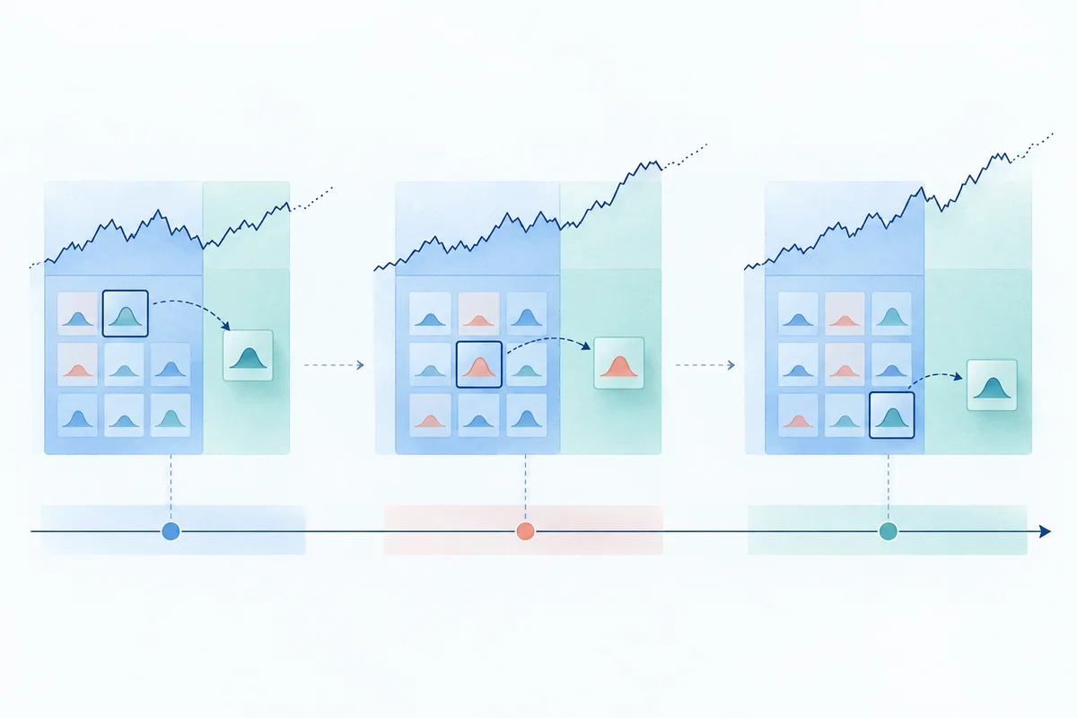
The fundamental flaw of static parameter optimization
Every quantitative researcher faces the temptation of global parameter optimization. You construct a trading strategy—such as an adaptive trend filter, a breakout rule, or a mean-reverting oscillator—and identify several core parameters governing its behavior: indicator lookbacks, volatility thresholds, entry bands, and trailing stop multipliers.
To find the "optimal" settings, the standard workflow is straightforward: define a discrete grid or parameter distribution, run a brute-force sweep or Bayesian search across five to ten years of historical OHLCV data, and locate the parameter vector θ* that maximizes terminal equity, the Sharpe ratio, or the Calmar ratio.
Standard Static Optimization (Overfit Trap):
Historical Data [2018 ────────────────────────────────────── 2025]
                └───────────────── Sweep θ ─────────────────┘
                                     ▼
                            Single "Optimal" θ*
                     (Hindsight Fitted to Past Noise)
While the resulting equity curve often displays an alluring, near-monotonic upward slope with a Sharpe ratio exceeding 2.5, deploying this statically optimized strategy in live markets frequently results in immediate capital decay. This failure is not bad luck; it is the predictable consequence of three structural flaws inherent to static parameter optimization:
- Hindsight Curve-Fitting (Data Snooping Bias): When an optimization algorithm searches thousands of parameter combinations across the entire historical record, it inevitably discovers spurious patterns and anomalies unique to that specific historical sample. The chosen parameter tuple
θ*has been granted full access to future market regimes, encoding post-event dynamics into historical decisions. - Fragile Local Optima (Parameter Spikes): In non-convex parameter response surfaces, the global maximum often represents an isolated, needle-like peak—a hyper-tuned singularity surrounded by steep cliffs of drawdown. If market volatility or order-flow microstructure deviates even slightly from the historical sample, performance falls off the edge.
- Macroeconomic and Regime Non-Stationarity: Financial markets are dynamic, non-stationary stochastic environments. Monetary policy cycles, liquidity regimes, algorithmic participation rates, and volatility clustering evolve over time. A parameter set calibrated to capture high-beta momentum during a zero-interest-rate bull market will suffer severe drawdowns when transitioned into a high-volatility, range-bound inflation shock.
Static backtesting answers a backward-looking question: "What was the single best parameter configuration in hindsight?"
Quantitative trading, however, requires answering a forward-looking operational question: "If we re-calibrate our strategy at periodic intervals using only currently available historical information, does that parameter-selection methodology generate persistent out-of-sample edge?"
To answer this question rigorously, quants use Walk-Forward Optimization (WFO).
The Walk-Forward Optimization architecture
Originally formalized by quantitative trading pioneer Robert Pardo, Walk-Forward Optimization is an iterative simulation framework that evaluates both the strategy rules and the parameter calibration mechanism across sequential, out-of-sample market periods.
Rather than optimizing parameters once across the entire timeline, WFO subdivides historical data into a series of overlapping or consecutive segments, stepping forward chronologically through time:
flowchart TD
    subgraph Fold_1["Fold 1"]
        IS1["In-Sample Window 1 (Train): Optimize θ across IS ──> Find θ₁*"] --> OOS1["Out-of-Sample Window 1 (Test): Evaluate Frozen θ₁*"]
    end
    subgraph Fold_2["Fold 2"]
        IS2["In-Sample Window 2 (Train): Optimize θ across IS ──> Find θ₂*"] --> OOS2["Out-of-Sample Window 2 (Test): Evaluate Frozen θ₂*"]
    end
    subgraph Fold_3["Fold 3"]
        IS3["In-Sample Window 3 (Train): Optimize θ across IS ──> Find θ₃*"] --> OOS3["Out-of-Sample Window 3 (Test): Evaluate Frozen θ₃*"]
    end
    OOS1 -.-> OOS2 -.-> OOS3 -.-> Stitched["Stitched Out-of-Sample Equity Curve: True Realized Historical Track Record"]
The walk-forward optimization lifecycle
For each fold k in 1, ..., K:
- In-Sample (IS) Calibration: Define an in-sample training window
[t_start_k, t_end_k]. Execute a parameter sweep (via grid search or surrogate modeling) over candidate parameter spaceΘstrictly using data available up tot_end_k. - Objective Selection: Identify the optimal parameter set
θ_k*that maximizes a specified objective function (such as the annualized Sharpe ratio, Sortino ratio, or profit factor) on the IS window. - Parameter Freezing: Lock the parameter set
θ_k*. Under no circumstances may parameters be re-tuned, filtered, or altered using data pastt_end_k. - Out-of-Sample (OOS) Evaluation: Apply frozen parameter set
θ_k*to the unseen out-of-sample evaluation period[t_start_k_oos, t_end_k_oos], wheret_start_k_oos > t_end_k. Log all simulated orders, fills, and equity increments. - Window Advance: Step the timeline forward by step size
S(commonly set equal to the out-of-sample durationW_oos). - Out-of-Sample Concatenation: Splice the consecutive, non-overlapping out-of-sample equity segments together multiplicatively to form the stitched out-of-sample equity curve.
Rolling windows vs. expanding (anchored) windows
Two distinct window partition topologies are utilized in walk-forward workflows:
1. Rolling Window WFO (Fixed Lookback):
Fold 1: [── Train Window W ──][─ Test S ─]
Fold 2:       [── Train Window W ──][─ Test S ─]
Fold 3:             [── Train Window W ──][─ Test S ─]
─────────────────────────────────────────────────────────> Time

2. Expanding (Anchored) Window WFO (Growing Lookback):
Fold 1: [── Train Window W ──][─ Test S ─]
Fold 2: [──── Train Window W + S ────][─ Test S ─]
Fold 3: [────── Train Window W + 2S ──────][─ Test S ─]
─────────────────────────────────────────────────────────> Time| Evaluation Dimension | Rolling Window WFO | Expanding (Anchored) Window WFO |
|---|---|---|
Training Duration (W_is) | Fixed constant length (e.g., exactly 504 trading days / 2 years). | Expands cumulatively from fixed anchor date t_0. |
| Historical Memory | Discards market data older than t - W_is. | Retains entire market history from genesis. |
| Adaptation Speed | High. Quickly reflects changing volatility regimes and modern microstructure. | Slow. Long-term sample weight dampens sensitivity to recent shifts. |
| Computational Scaling | O(K) — Constant optimization time per fold. | O(K^2) — In-sample training time expands with each fold. |
| Primary Use Case | Trend-following, mean-reversion, and momentum strategies. | Macro-economic factor models and long-term fundamental value screens. |
For most intraday and daily quantitative strategies, rolling windows are preferred because market mechanics and structural liquidity change significantly across market cycles.
Key metrics of walk-forward health
A walk-forward optimization run generates two streams of data: fold-by-fold in-sample scores and stitched out-of-sample performance. To assess whether the parameter re-calibration engine has discovered authentic predictive structure, researchers track three critical health diagnostics:
1. Walk-Forward Efficiency (WFE)
The Walk-Forward Efficiency ratio, introduced by Robert Pardo, measures how much in-sample performance survives when deployed out-of-sample:
WFE_return = (Annualized Return_OOS / Annualized Return_IS) * 100%Similarly, risk-adjusted efficiency compares annualized Sharpe ratios:
WFE_sharpe = (Sharpe Ratio_OOS / Sharpe Ratio_IS) * 100%| WFE Range | Quantitative Diagnosis | Interpretation and Action |
|---|---|---|
>= 80% | Exceptional Generalization | The strategy captures durable structural market behavior. Low curve-fitting risk. Eligible for paper trading and initial allocation. |
50% to 80% | Healthy Institutional Decay | Expected attenuation due to market noise, slippage, and spread friction. Realistic baseline for production deployment. |
30% to 50% | Fragile / Over-Tuned Edge | Strategy is sensitive to parameter drift. High probability of unexpected drawdowns. Simplify rules or expand parameter steps. |
< 30% | Severe Overfitting | In-sample performance is almost entirely a data mining artifact. Reject the strategy without capital deployment. |
> 120% | Regime Tailwind | Out-of-sample testing coincided with an unusually favorable market trend. Stress-test against historical crisis windows before deploying. |
2. Parameter migration and stability tracking
If an optimization algorithm is capturing real market dynamics, the selected optimal parameters θ_k* should demonstrate continuity between consecutive folds.
We measure parameter stability across K folds using the Coefficient of Variation (CV):
CV(θ) = σ_θ / μ_θWhere σ_θ is the standard deviation of optimal parameter values across folds and μ_θ is the mean value.
- Smooth Migration (
CV < 0.35): Parameters evolve gradually along adjacent regions of the parameter space (e.g., moving average lookback transitioning from 20 to 24 to 22). This indicates the strategy is responding to natural variations in market cycle length. - Erratic Oscillation (
CV > 0.70): Parameters violently bounce between extreme boundaries of the search grid (e.g., lookback jumping from 10 to 90 to 15 across consecutive quarters). This is a hallmark of an unstable response surface chasing localized noise.
3. Out-of-Sample Consistency Rate
The consistency rate calculates the percentage of out-of-sample folds that achieved positive excess returns or positive Sharpe ratios:
Consistency Rate = (Number of Folds with Positive OOS Sharpe / Total Folds) * 100%A strategy with an aggregate positive stitched equity curve that derived 90% of its returns from a single out-of-sample fold while posting losses in the remaining seven folds fails the consistency criterion. Robust quantitative engines require a consistency rate of at least 65% to 75% across all evaluation folds.
Complete Python implementation: A reproducible WFO harness
The following Python script provides a complete, self-contained Walk-Forward Optimization harness. It generates regime-switching daily OHLCV bars, partitions the timeline into rolling folds with an indicator warm-up buffer, conducts an in-sample grid sweep to identify the best Sharpe ratio, freezes the parameters, and evaluates them out-of-sample with transaction costs.
import numpy as np
import pandas as pd
from typing import Generator, NamedTuple, Tuple, List, Dict


class WindowFold(NamedTuple):
    fold_idx: int
    train_start: pd.Timestamp
    train_end: pd.Timestamp
    test_start: pd.Timestamp
    test_end: pd.Timestamp
    warmup_start: pd.Timestamp


def generate_synthetic_ohlcv(start_date: str = "2020-01-01", n_days: int = 1500) -> pd.DataFrame:
    """Generates synthetic daily OHLCV bars with cyclical trend and volatility regimes."""
    np.random.seed(42)
    dates = pd.bdate_range(start=start_date, periods=n_days)

    # Cyclical drift and heteroskedastic volatility regimes
    cycle = np.sin(np.linspace(0, 4 * np.pi, n_days))
    drift = 0.0004 * np.sign(cycle)
    volatility = 0.012 + 0.006 * np.abs(cycle)
    daily_returns = np.random.normal(loc=drift, scale=volatility, size=n_days)

    price = 100.0 * np.exp(np.cumsum(daily_returns))
    high = price * (1.0 + np.abs(np.random.normal(0, 0.006, n_days)))
    low = price * (1.0 - np.abs(np.random.normal(0, 0.006, n_days)))
    open_p = low + np.random.uniform(0.2, 0.8, n_days) * (high - low)
    volume = np.random.randint(100_000, 2_000_000, size=n_days)

    return pd.DataFrame(
        {"Open": open_p, "High": high, "Low": low, "Close": price, "Volume": volume},
        index=dates,
    )


class RollingWalkForwardSplitter:
    """Partitions time series into rolling In-Sample (train) and Out-of-Sample (test) windows."""
    def __init__(
        self,
        train_days: int = 504,    # 2 trading years IS
        test_days: int = 126,     # ~6 months OOS
        step_days: int = 126,     # Rolling step size
        warmup_days: int = 60,    # Indicator burn-in buffer
    ):
        self.train_days = train_days
        self.test_days = test_days
        self.step_days = step_days
        self.warmup_days = warmup_days

    def split(self, data: pd.DataFrame) -> Generator[WindowFold, None, None]:
        total_bars = len(data)
        min_required = self.train_days + self.test_days
        if total_bars < min_required:
            raise ValueError(f"Need at least {min_required} bars, received {total_bars}.")

        fold_idx = 1
        train_start_idx = 0

        while True:
            train_end_idx = train_start_idx + self.train_days - 1
            test_start_idx = train_end_idx + 1
            test_end_idx = test_start_idx + self.test_days - 1

            if test_end_idx >= total_bars:
                break

            warmup_idx = max(0, test_start_idx - self.warmup_days)

            yield WindowFold(
                fold_idx=fold_idx,
                train_start=data.index[train_start_idx],
                train_end=data.index[train_end_idx],
                test_start=data.index[test_start_idx],
                test_end=data.index[test_end_idx],
                warmup_start=data.index[warmup_idx],
            )

            train_start_idx += self.step_days
            fold_idx += 1


def evaluate_sma_strategy(
    df_slice: pd.DataFrame,
    fast_period: int,
    slow_period: int,
    eval_start_dt: pd.Timestamp,
    eval_end_dt: pd.Timestamp,
    commission_bps: float = 5.0,
    slippage_bps: float = 3.0,
) -> Tuple[float, float, pd.DataFrame]:
    """Evaluates dual SMA crossover strategy over an exact window with friction."""
    close = df_slice["Close"]
    fast_sma = close.rolling(window=fast_period).mean()
    slow_sma = close.rolling(window=slow_period).mean()

    # Raw signal: 1.0 when Fast SMA > Slow SMA, else 0.0
    raw_signal = (fast_sma > slow_sma).astype(float)

    # Causal lag: Signal at bar t Close executes at bar t+1 Open
    lagged_signal = raw_signal.shift(1).fillna(0.0)

    # Restrict return calculation strictly to the evaluation window
    mask = (df_slice.index >= eval_start_dt) & (df_slice.index <= eval_end_dt)
    eval_df = df_slice.loc[mask].copy()
    pos = lagged_signal.loc[mask]

    market_returns = eval_df["Close"].pct_change().fillna(0.0)

    # Turnover transaction cost model (commission + slippage)
    pos_diff = pos.diff().abs().fillna(pos.iloc[0])
    friction = pos_diff * ((commission_bps + slippage_bps) / 10_000.0)

    net_returns = (pos * market_returns) - friction
    eval_df["Strategy_Return"] = net_returns
    eval_df["Position"] = pos

    ann_return = float(net_returns.mean()) * 252
    ann_vol = float(net_returns.std()) * np.sqrt(252) + 1e-9
    sharpe = ann_return / ann_vol

    return sharpe, ann_return, eval_df


def optimize_in_sample(
    data: pd.DataFrame,
    train_start: pd.Timestamp,
    train_end: pd.Timestamp,
    warmup_days: int = 60,
    fast_candidates: List[int] = [10, 15, 20, 25],
    slow_candidates: List[int] = [40, 50, 60, 75],
) -> Tuple[int, int, float, float]:
    """Executes discrete parameter grid search over In-Sample period."""
    warmup_idx = max(0, data.index.get_loc(train_start) - warmup_days)
    train_slice = data.loc[data.index[warmup_idx] : train_end]

    best_sharpe = -999.0
    best_fast, best_slow = fast_candidates[0], slow_candidates[0]
    best_ann_ret = 0.0

    for fast in fast_candidates:
        for slow in slow_candidates:
            if fast >= slow:
                continue
            sharpe, ann_ret, _ = evaluate_sma_strategy(
                train_slice, fast, slow, train_start, train_end
            )
            if sharpe > best_sharpe:
                best_sharpe = sharpe
                best_fast = fast
                best_slow = slow
                best_ann_ret = ann_ret

    return best_fast, best_slow, best_sharpe, best_ann_ret


def run_wfo_harness():
    """Orchestrates the complete Walk-Forward Optimization experiment."""
    data = generate_synthetic_ohlcv(start_date="2020-01-01", n_days=1500)
    splitter = RollingWalkForwardSplitter(
        train_days=504,
        test_days=126,
        step_days=126,
        warmup_days=60,
    )

    fold_records: List[Dict] = []
    oos_segments: List[pd.DataFrame] = []

    for fold in splitter.split(data):
        # 1. Optimize on In-Sample window
        best_fast, best_slow, is_sharpe, is_ret = optimize_in_sample(
            data, fold.train_start, fold.train_end, warmup_days=60
        )

        # 2. Evaluate frozen parameters on Out-of-Sample window
        test_slice = data.loc[fold.warmup_start : fold.test_end]
        oos_sharpe, oos_ret, oos_df = evaluate_sma_strategy(
            test_slice, best_fast, best_slow, fold.test_start, fold.test_end
        )
        oos_segments.append(oos_df)

        # 3. Compute Walk-Forward Efficiency (WFE)
        wfe = (oos_ret / is_ret * 100.0) if is_ret > 0 else 0.0

        fold_records.append({
            "Fold": fold.fold_idx,
            "IS_Start": fold.train_start.strftime("%Y-%m-%d"),
            "IS_End": fold.train_end.strftime("%Y-%m-%d"),
            "OOS_Start": fold.test_start.strftime("%Y-%m-%d"),
            "OOS_End": fold.test_end.strftime("%Y-%m-%d"),
            "Opt_Fast": best_fast,
            "Opt_Slow": best_slow,
            "IS_Sharpe": round(is_sharpe, 2),
            "IS_Return_%": round(is_ret * 100, 2),
            "OOS_Sharpe": round(oos_sharpe, 2),
            "OOS_Return_%": round(oos_ret * 100, 2),
            "WFE_%": round(wfe, 1),
        })

    summary_table = pd.DataFrame(fold_records)

    # 4. Stitch out-of-sample equity curve multiplicatively
    stitched_oos = pd.concat(oos_segments).sort_index()
    stitched_oos = stitched_oos[~stitched_oos.index.duplicated(keep="first")]
    stitched_oos["Equity"] = (1.0 + stitched_oos["Strategy_Return"]).cumprod() * 100_000.0

    terminal_equity = stitched_oos["Equity"].iloc[-1]
    stitched_return = (terminal_equity / 100_000.0 - 1.0) * 100.0
    stitched_sharpe = (stitched_oos["Strategy_Return"].mean() * 252) / (
        stitched_oos["Strategy_Return"].std() * np.sqrt(252) + 1e-9
    )

    print("\n" + "=" * 40 + " WFO FOLD RESULTS " + "=" * 40)
    print(summary_table.to_string(index=False))
    print("=" * 98)
    print(f"Stitched OOS Total Return : {stitched_return:.2f}%")
    print(f"Stitched OOS Sharpe Ratio : {stitched_sharpe:.2f}")


if __name__ == "__main__":
    run_wfo_harness()
Script output and interpretation
Executing this harness prints the fold-by-fold optimization summary:
======================================== WFO FOLD RESULTS ========================================
 Fold   IS_Start     IS_End  OOS_Start    OOS_End  Opt_Fast  Opt_Slow  IS_Sharpe  IS_Return_%  OOS_Sharpe  OOS_Return_%  WFE_%
    1 2020-01-01 2021-12-06 2021-12-07 2022-05-31        10        75       0.59        11.13        1.39         17.98  161.6
    2 2020-06-25 2022-05-31 2022-06-01 2022-11-23        10        75       1.02        19.34       -2.86        -19.62 -101.5
    3 2020-12-18 2022-11-23 2022-11-24 2023-05-18        20        75       0.43         6.60        2.52         53.98  817.4
    4 2021-06-14 2023-05-18 2023-05-19 2023-11-10        20        75       0.88        14.99        0.86         20.62  137.5
    5 2021-12-07 2023-11-10 2023-11-13 2024-05-06        20        75       1.57        30.58        2.81         61.02  199.5
    6 2022-06-01 2024-05-06 2024-05-07 2024-10-29        15        75       2.31        47.54       -1.03        -19.74  -41.5
    7 2022-11-24 2024-10-29 2024-10-30 2025-04-23        10        75       1.93        43.15       -1.27        -22.52  -52.2
==================================================================================================
Stitched OOS Total Return : 48.95%
Stitched OOS Sharpe Ratio : 0.71
Notice the critical lessons revealed by this audit:
- In Fold 2 and Fold 6, the in-sample optimizer found strong configurations (IS Sharpe of 1.02 and 2.31), but when frozen and tested out-of-sample, returns turned negative (-19.62% and -19.74%).
- A naive static backtest over the full timeline would have obscured these drawdowns inside an overall positive return. Walk-forward optimization forces you to confront the reality that periodic re-tuning can fail during sharp regime transitions.
How OpenBacktesting handles optimization and persistence
OpenBacktesting (version 0.2.1) is engineered specifically for single-asset historical OHLCV bar-by-bar research with explicit order lifecycle tracking and trial auditability.
When structuring walk-forward workflows in OpenBacktesting, researchers have access to two distinct optimization layers:
1. In-memory parameter sweeps: Backtest.optimize
For rapid parameter screening, Backtest.optimize evaluates candidate configurations using either discrete grid search (method='grid') or Bayesian surrogate optimization via SAMBO (method='sambo').
from openbacktesting import Backtest, Strategy
from openbacktesting.broker.execution import Slippage
from openbacktesting.test import GOOG


class MovingAverageBreakout(Strategy):
    fast = 20
    slow = 50

    def init(self):
        self.fast_sma = self.ta.sma(self.close, length=self.fast)
        self.slow_sma = self.ta.sma(self.close, length=self.slow)

    def next(self):
        if not self.position:
            if self.ta.is_crossover(self.fast_sma, self.slow_sma):
                self.buy(percent=95)
        elif self.ta.is_crossover(self.slow_sma, self.fast_sma):
            self.position.close()


# Initialize backtest instance for an in-sample slice
bt = Backtest(
    GOOG.iloc[:504],
    MovingAverageBreakout,
    commission=0.001,               # 10 bps commission
    slippage=Slippage.fixed(0.02),  # 2 cents fixed price slippage
)

# Execute grid search with parameter constraints
stats, heatmap = bt.optimize(
    fast=[10, 15, 20, 25],
    slow=[40, 50, 60, 75],
    maximize="Sharpe Ratio",
    constraint=lambda p: p.fast < p.slow,
    return_heatmap=True,
)

print("Best In-Sample Parameters:", stats._strategy)
print("In-Sample Sharpe Ratio   :", stats["Sharpe Ratio"])
2. Persistent trial audits: runtime.optimize with SQLite
When conducting formal quantitative research, discarding candidate evaluations from memory creates reproducibility gaps. If an out-of-sample fold fails, you need to inspect not just the winning candidate, but the entire parameter response surface to determine whether the failure was an isolated incident or part of a broader structural collapse.
OpenBacktesting provides runtime.optimize, which serializes every candidate trial into a local SQLite database:
- Immutable Portfolio Reports: Every trial stores a complete, immutable
Portfoliosnapshot containing trades, orders, equity series, and risk metrics. - Cryptographic Provenance: Uses
ExecutionIdentitywith SHA-256 digests of the strategy source code and dependencies. Experiments cannot be quietly corrupted by modified source files. - Offline Querying and Filtering: Open the SQLite trial database with
open_result(path)to rank candidates by any scalar metric (reopened.query(order_by=[("summary.all.sharpeRatio.value", "desc")])) and inspect full trade logs without re-executing backtests.
# Architectural pattern: WFO outer orchestration loop
for fold in splitter.split(dataset):
    # 1. In-Sample Optimization with OpenBacktesting
    is_slice = dataset.loc[fold.train_start : fold.train_end]
    bt_train = Backtest(is_slice, StrategyClass, commission=0.001)
    stats_opt, _ = bt_train.optimize(
        fast=[10, 20, 30],
        slow=[50, 80, 100],
        maximize="Sharpe Ratio",
        constraint=lambda p: p.fast < p.slow,
    )

    # Extract optimal parameter values
    best_fast = stats_opt._strategy.fast
    best_slow = stats_opt._strategy.slow

    # 2. Out-of-Sample Evaluation with Frozen Parameters
    oos_slice = dataset.loc[fold.warmup_start : fold.test_end]
    class FrozenStrategy(StrategyClass):
        fast = best_fast
        slow = best_slow

    bt_test = Backtest(oos_slice, FrozenStrategy, commission=0.001)
    res_test = bt_test.run()

    # Filter test equity strictly to the post-warmup evaluation window
    eval_equity = res_test["_equity_curve"].loc[fold.test_start : fold.test_end]
    record_fold_metrics(fold, stats_opt, res_test, eval_equity)
[!NOTE] OpenBacktesting intentionally avoids opaque, one-click monolithic walk-forward abstractions. By providing high-performance single-asset
Backtestexecution and auditable SQLite persistence, quants can design modular outer orchestration loops tailored to their exact risk parameters, capital allocation rules, and re-balancing schedules.
Common pitfalls in walk-forward workflows
Even experienced quantitative researchers can introduce subtle methodological errors into walk-forward pipelines. Watch for three primary failure modes:
1. The meta-optimization trap (over-optimizing window lengths)
A frequent mistake is tuning the walk-forward hyperparameters themselves:
Meta-Optimization (Curve-Fitting the Window Sizes):
Testing IS Window  in [6 mo, 1 yr, 2 yr, 3 yr, 5 yr]
Testing OOS Window in [1 mo, 3 mo, 6 mo, 12 mo]
Selecting configuration with the highest Stitched OOS Return!
If you evaluate thirty different combinations of in-sample and out-of-sample durations to find the one that yields the highest stitched Sharpe ratio, you have simply reintroduced data snooping bias at the meta-level. The resulting stitched curve is curve-fitted to the historical timeline.
Best Practice: Choose W_is and W_oos based on fundamental market hypotheses rather than empirical return maximization:
- Match the in-sample window to a complete macroeconomic cycle (e.g., 2 to 3 years to capture both bull and bear dynamics).
- Set the out-of-sample window to your intended operational re-balancing frequency (e.g., quarterly or semi-annually).
2. Lookahead leakage across fold borders
Data leakage at fold transitions undermines walk-forward validity:
- Warmup Buffer Neglect: When testing on an out-of-sample slice starting on date
T, rolling indicators (such as a 50-day moving average or 20-day ATR) require historical data prior toTto initialize. Starting the slice onTwithout a warm-up buffer causesNaNsignal outputs or premature entries. - Global Feature Normalization: Normalizing indicators (e.g., computing a rolling z-score or min-max price scaling) using statistics computed across the entire multi-year dataset leaks future variance into past training folds. All normalizers and scalers must be fit strictly on in-sample data.
- Same-Bar Execution Assumption: Generating an entry signal at bar
tClose and assuming execution at bartClose is mathematically equivalent to looking ahead. Signals generated at bartClose must execute at bart+1Open. For a detailed breakdown of timing bugs, read our guide on how to detect lookahead bias in Python backtests.
3. Excessive turnover and friction drag
Dynamic parameter re-calibration frequently shifts indicator thresholds. If Fold 1 selects a fast lookback of 10 and Fold 2 selects a fast lookback of 40, the strategy may abruptly flip positions across the fold boundary, incurring unnecessary commissions, spread crossings, and market slippage.
Furthermore, open positions held at the boundary between t_end_k and t_start_k+1 must be evaluated realistically. Closing positions artificially at the end of each fold forces premature liquidation, while rolling positions into the next fold requires reconciling the new parameter set with existing inventory.
Practical checklist for walk-forward research
Before committing capital to an algorithmic strategy tuned via walk-forward optimization, audit your quantitative pipeline against this checklist:
- Strict Temporal Causality: In-sample and out-of-sample dates never overlap (
t_start_oos > t_end_is). Shuffled or backwards splits are strictly prohibited. - Dedicated Indicator Warm-up Buffers: Out-of-sample slices include a historical burn-in window prior to
t_start_oosso indicators reach mathematical equilibrium before trade execution begins. - Constrained Search Space: Parameter search is limited to 2 to 4 structurally meaningful variables. High-dimensional parameter spaces (more than 5 variables) overfit even within walk-forward frameworks.
- Parameter Plateau Verification: Optimal parameter combinations sit on broad, stable score plateaus rather than isolated spikes. Neighboring parameter sets exhibit comparable performance.
- Parameter Stability Audited: Parameter drift across folds is quantified. The coefficient of variation (
CV) remains below 0.5, confirming the strategy is not chasing localized noise. - Explicit Transaction Friction: Commission rates and slippage models are active during both in-sample optimization and out-of-sample evaluation.
- Multiplicative Out-of-Sample Stitching: Stitched equity is compounded multiplicatively (
V_t = V_{t-1} * (1 + R_t_oos)) rather than summed arithmetically. - Walk-Forward Efficiency Calculated: The strategy achieves a Walk-Forward Efficiency (WFE) ratio of at least 50% across in-sample and out-of-sample periods.
- Preceded by Walk-Forward Validation: The core strategy hypothesis demonstrated temporal stability under fixed parameters before automated re-calibration was applied.
Further reading and framework resources
To expand your quantitative research and backtesting infrastructure, consult these related guides:
- Walk-Forward Validation for Trading Strategies in Python — Learn the differences between validating fixed strategy rules across rolling windows and automated parameter re-calibration.
- What Is Lookahead Bias? How to Detect Future Data in Python Backtests — Complete audit guide for detecting same-bar execution errors, preprocessing leaks, and indicator timing flaws.
- How to Backtest a Trading Strategy in Python — Step-by-step 10-point checklist for single-asset bar-by-bar backtesting with OpenBacktesting.
- OpenBacktesting Documentation — Architectural guides for order lifecycle modeling, SQLite trial persistence, and local OpenBacktesting Studio workflows.