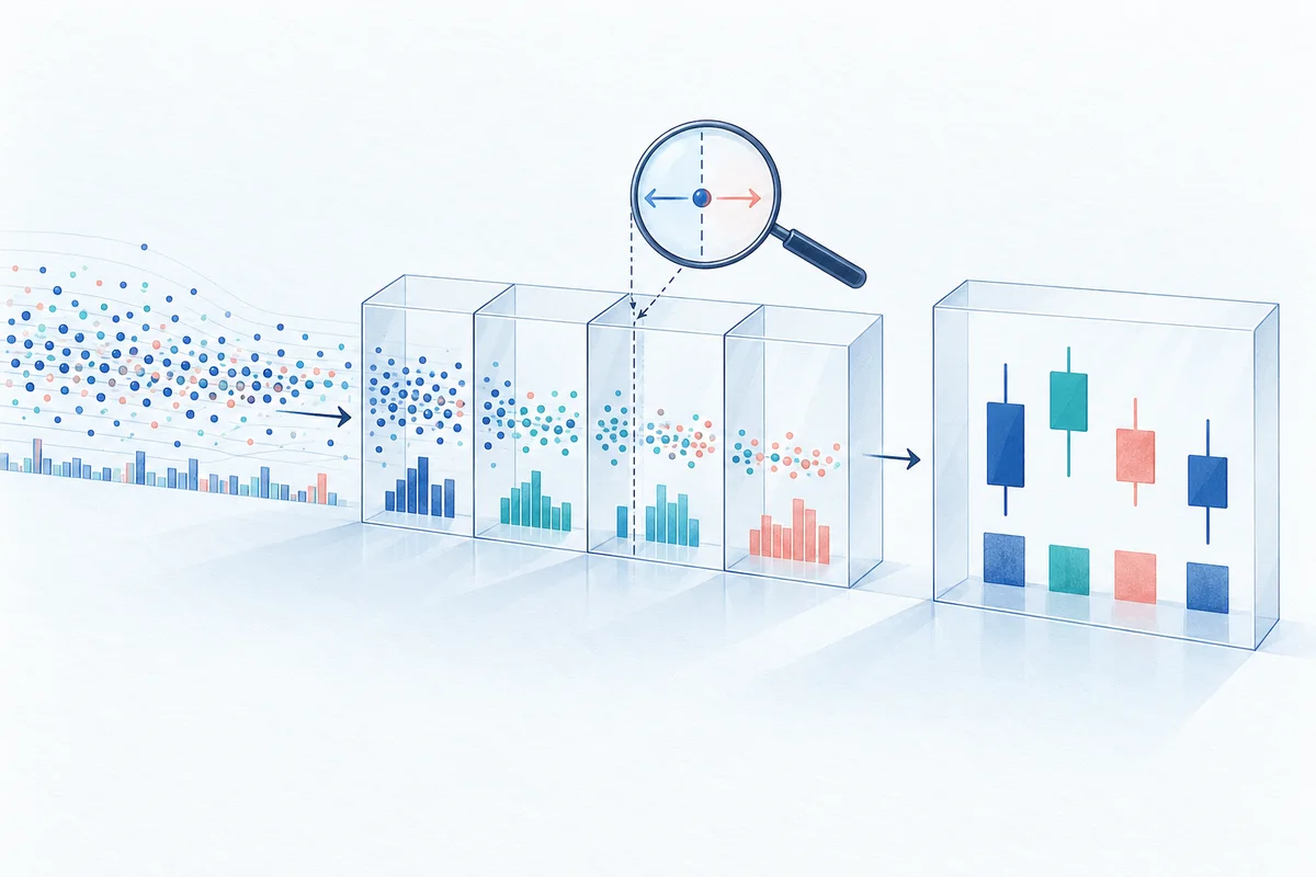
The high-frequency dilemma: Why tick backtesting is deceptively complex
In quantitative strategy development, many researchers assume that migrating from minute or daily bars to raw tick data automatically yields institutional-grade fidelity. The intuition seems unassailable: if a backtest evaluates every individual trade as it occurs on the exchange matching engine, execution assumptions should reflect physical reality rather than the coarse approximations of synthetic OHLCV candles.
In practice, working with backtrader tick data introduces subtle architectural hazards that frequently invalidate research findings. High-frequency tick feeds are not simply smaller bars; they represent an entirely different data regime characterized by asynchronous event arrivals, microsecond timestamps, bid-ask bouncing, and complex boundary conditions.
When ingesting tick data into an event-driven engine like Backtrader, researchers encounter three critical failure modes:
- Semantic data confusion: Conflating executed transaction ticks (trade ticks) with top-of-book quotes (Best Bid and Offer, or BBO updates), resulting in distorted trading volume and phantom price extremes.
- Boundary and dispatch distortion: Misaligning interval edges (
bar2edge, left-closed versus right-closed intervals) and misunderstanding when Backtrader actually finalizes and dispatches a resampled bar toStrategy.next(). - CPython memory exhaustion: Attempting to iterate hundreds of millions of tick objects through pure Python line buffers, resulting in Out-Of-Memory (OOM) crashes and 100x execution slowdowns.
flowchart TD
    A["Raw Market Feed Stream"] --> B{"Event Classifier"}
    B -->|"Quote Update (BBO)"| C["Resting Liquidity Depth\n(Discard for Standard Bars)"]
    B -->|"Trade Print (Execution)"| D["Valid Trade Tick\n(Timestamp, Price, Size)"]
    D --> E["Aggregation Bucket [T_start, T_end)"]
    E --> F["Running High / Low Extrema"]
    E --> G["Cumulative Volume Sum"]
    F & G --> H{"Subsequent Tick >= T_end?"}
    H -->|"No"| E
    H -->|"Yes: Boundary Event"| I["Finalize Previous Bar (OHLCV)"]
    I --> J["Dispatch to Strategy.next()"]
This guide provides a comprehensive technical walkthrough for loading, resampling, and auditing tick data in Backtrader. We dissect the fundamental difference between trade prints and quote updates, demonstrate how to configure custom sub-second data feeds, verify exact bar boundary aggregation through a micro-sample audit, and examine why production quantitative workflows pre-aggregate ticks into validated bars using vectorized tools before conducting strategy research.
Market microstructure foundations: Trade ticks vs quote ticks (BBO)
Before writing a single line of ingestion code, you must establish an unambiguous definition of what constitutes a "tick." In electronic financial markets, exchanges stream two fundamentally distinct categories of tick-level messages:
Market Data Stream
├── 1. Trade Ticks (Time & Sales Tape):
│      Executed transactions between aggressive market orders and passive limit orders.
│      Attributes: Trade ID, Timestamp, Executed Price, Executed Volume, Aggressor Side.
│
└── 2. Quote Ticks (Top-of-Book / Level 1 BBO):
       Modifications to resting passive liquidity at the Best Bid and Best Offer.
       Attributes: Timestamp, Bid Price, Bid Size, Ask Price, Ask Size.
Why feeding quote ticks into OHLCV bars corrupts your model
A frequent mistake when configuring a backtrader tick data pipeline is ingesting a combined trade-and-quote feed without filtering out quote modifications. In high-frequency equity and crypto markets, quote updates outnumber executed trades by anywhere from 10:1 to 100:1.
Passing quote updates into a standard OHLCV aggregator introduces two fatal mathematical errors:
1. The phantom volume catastrophe
In a trade tick, the size attribute represents real shares or contracts that exchanged hands (V_traded). Volume is strictly additive:
Bar Volume = ∑ Size(i) for all trades i in [T_start, T_end)In a quote tick, the size attribute represents resting queue depth (Q_bid or Q_ask). If a market maker posts a limit order to buy 500 shares at $150.00, updates the price to $150.01 two milliseconds later, and then cancels it, zero shares were traded.
If your ingestion parser maps the quote's size field to Backtrader's volume line, those 500 shares are counted repeatedly on every update. Over a 5-minute interval, a single resting order modified 20 times appears as 10,000 shares of fictitious trading volume. Volume-weighted indicators like VWAP, Volume Profiles, and OBV become completely meaningless.
2. Spurious price extremes and bid-ask bouncing
Quote prices flicker continuously across the bid-ask spread. If the market is quoted $150.00 bid / $150.10 ask, and an aggregator indiscriminately ingests both bid and ask quote ticks as price events, the resulting candle registers an interval High of $150.10 and Low of $150.00—even if not a single trade occurred within that spread.
In low-liquidity instruments with wide spreads, this artificial price widening creates synthetic volatility spikes, triggering false breakout entries and phantom stop-out executions.
| Characteristic | Trade Ticks (Time & Sales) | Quote Updates (Level 1 BBO) |
|---|---|---|
| Physical Reality | Executed transaction between counterparties | Change in resting passive order queue |
| Frequency Ratio | Baseline ($1\times$) | Extremely dense ($10\times$ to $100\times$ trade volume) |
| Volume Semantics | Real additive volume ($V \ge 1$) | Resting capacity depth (not additive) |
| High / Low Validity | Actual traded prices | Unexecuted bid/ask extremes (spread noise) |
| Aggregation Target | Valid input for tick OHLCV bars | Requires specialized order book reconstruction |
| Backtrader Suitability | Native line buffer support | Requires custom order book data structures |
[!IMPORTANT] Always verify that your tick data source contains pure transaction prints (often labeled
trades.csvorTimeAndSales) rather than top-of-book depth updates (quotes.csvorBBO). If your data vendor delivers a merged stream, pre-filter records whererecord_type == 'trade'before feeding them into Backtrader.
Ingesting tick data into Backtrader: Sub-second CSV feeds
Backtrader provides native architectural support for tick resolution through bt.TimeFrame.Ticks. However, its default GenericCSVData parser expects second- or minute-level timestamps formatted as YYYY-MM-DD HH:MM:SS.
Real-world trade ticks require sub-second precision (milliseconds or microseconds, formatted as %Y-%m-%d %H:%M:%S.%f). To ingest these records without losing temporal granularity, we must subclass GenericCSVData and configure Backtrader's datetime parsing mechanisms.
Designing a sub-second trade tick feed
In a standard trade tick record, each row represents a single instantaneous print:
timestamp: Sub-second execution timestamp (e.g.,2026-01-11 09:30:04.120000).price: Executed transaction price.size: Executed contract or share quantity.side: Optional aggressor flag (Buy,Sell, orNeutral).
Because Backtrader's internal Lines architecture always requires six core components (datetime, open, high, low, close, volume), a single trade print is represented as a degenerate candle where:
Open = High = Low = Close = Trade Price
Volume = Traded Size
Here is the production implementation of a custom sub-second tick parser:
from datetime import datetime
import backtrader as bt

class SubsecondCSVData(bt.feeds.GenericCSVData):
    """
    Custom CSV data feed for sub-second trade tick records.
    Maps a single trade print into Backtrader's line structure.
    """
    params = (
        ('nullvalue', float('NaN')),
        ('dtformat', '%Y-%m-%d %H:%M:%S.%f'),
        ('tmformat', '%H:%M:%S.%f'),
        ('timeframe', bt.TimeFrame.Ticks),
        ('compression', 1),
        ('datetime', 0),    # Column 0: Timestamp
        ('open', 1),        # Column 1: Price
        ('high', 1),        # Column 1: Price (degenerate tick)
        ('low', 1),         # Column 1: Price (degenerate tick)
        ('close', 1),       # Column 1: Price (degenerate tick)
        ('volume', 2),      # Column 2: Trade Size
        ('openinterest', -1)# Not present in standard trade tape
    )
For deeper architectural details on extending Backtrader data schemas, refer to our comprehensive guide on creating a Backtrader custom data feed.
Resampling tick data to bars in Cerebro: Engine mechanics
Once tick data is loaded into Backtrader, researchers typically aggregate raw prints into higher-granularity intervals—such as 1-minute, 5-minute, or 15-minute bars—for indicator computation and signal generation. This process is known as Backtrader tick resampling.
Backtrader provides two primary resampling methods within bt.Cerebro:
cerebro.resampledata(...): Ingests a granular feed and aggregates it dynamically during execution, replacing the original feed.cerebro.replaydata(...): Delivers each intermediate tick update within the forming bar to simulate intra-bar price action, finalizing the bar when the interval completes.
Configuring dynamic tick resampling
To resample raw ticks into 1-minute OHLCV bars, pass the tick feed to cerebro.resampledata with explicit boundary parameters:
import backtrader as bt

def setup_cerebro_resampling(tick_datapath: str) -> bt.Cerebro:
    cerebro = bt.Cerebro()

    # Ingest raw trade ticks
    raw_tick_feed = SubsecondCSVData(
        dataname=tick_datapath,
        timeframe=bt.TimeFrame.Ticks,
        compression=1
    )

    # Resample ticks to 1-Minute bars
    cerebro.resampledata(
        raw_tick_feed,
        timeframe=bt.TimeFrame.Minutes,
        compression=1,
        bar2edge=True,      # Align bar timestamps to round clock edges
        adjtime=True,       # Adjust bar timestamp to the edge
        rightedge=False     # Left-closed interval timestamping
    )

    return cerebro
Dynamic tick resampling vs multi-timeframe synchronization
It is crucial to distinguish tick-to-bar resampling from the multi-timeframe synchronization discussed in our analysis of Backtrader Multiple Timeframes.
When synchronizing daily and hourly feeds in Backtrader, both feeds arrive as pre-formed, discrete bars. The engine's primary challenge is temporal alignment: ensuring the strategy does not evaluate a daily bar's closing price until the final hourly bar of that day has completed, thereby preventing lookahead bias.
In contrast, tick resampling processes an unaligned, stochastic point process. Trade ticks arrive at non-deterministic sub-second intervals:
Tick 1: 09:30:04.120 -> Tick 2: 09:30:12.450 -> Tick 3: 09:30:58.910 -> Tick 4: 09:33:14.050Backtrader's internal bt.filters.Resampler must maintain running state variables across asynchronous arrivals:
open: Recorded from the first tick inside the bucket.high: Updated asmax(running_high, tick_price).low: Updated asmin(running_low, tick_price).close: Continuously overwritten by incomingtick_price.volume: Accumulated asrunning_volume + tick_size.
The bar cannot be finalized until an event signals that the interval has officially closed.
Bar boundary verification: Timestamps, closures, and dispatch lag
The most common source of discrepancy between Backtrader backtests and external data benchmarks lies in bar boundary semantics. If two systems disagree by even one millisecond on which bucket a trade belongs to, their resulting OHLCV values will diverge.
1. Left-closed vs right-closed interval boundaries
Standard quantitative convention models time intervals as left-closed, right-open:
[T_start, T_end) = {t ∈ Time | T_start ≤ t < T_end}For a 1-minute bar starting at 09:30:00:
- A tick stamped
09:30:00.000000belongs to the09:30bar. - A tick stamped
09:30:59.999999belongs to the09:30bar. - A tick stamped
09:31:00.000000belongs to the09:31bar.
In Backtrader's resampledata, the parameter bar2edge=True forces the aggregation boundaries to snap to clean calendar intervals (e.g., 09:30:00, 09:31:00, 09:32:00) rather than measuring relative duration from the first tick's arbitrary timestamp.
The rightedge parameter governs timestamp labeling:
rightedge=False(Standard): Labels the bar with its opening boundary (09:30:00).rightedge=True: Labels the bar with its closing boundary (09:31:00).
Researchers must remain consistent across their entire pipeline. Labeling a bar 09:30:00 while allowing the strategy to trade on its close at 09:30:01 is a severe form of lookahead bias.
2. The dispatch lag problem in historical tick streams
In a live trading environment, a hardware clock triggers bar completion exactly at 09:31:00.000000. In a historical backtest, however, Backtrader possesses no independent clock. Time advances strictly through incoming data records.
This creates a critical behavioral artifact known as dispatch lag:
Historical Event Timeline:
09:30:04.120 [Tick 1] -> Bar 09:30 opened
09:30:58.910 [Tick 6] -> Last tick in 09:30 window
... No trades occur for 3 minutes (illiquid pause) ...
09:34:10.250 [Tick 7] -> First tick of new interval!
                         ==> ONLY NOW does Backtrader finalize Bar 09:30!
                         ==> Strategy.next() for Bar 09:30 executes at 09:34:10!
If an asset experiences low trading volume, Backtrader cannot know that the 09:30 bar has completed until it observes Tick 7 arriving at 09:34:10. Only upon encountering a timestamp greater than or equal to 09:31:00.000000 does the resampler seal the 09:30 bar and pass it to Strategy.next().
3. Missing bars and zero-volume gaps
What happens to the intervals between 09:31:00 and 09:34:00 where zero trades occurred?
By default, Backtrader's resampler skips intervals that contain no ticks. It does not automatically generate synthetic zero-volume bars unless explicitly instructed.
This creates a non-uniform time series:
bar[0]=09:30:00bar[1]=09:34:00(Gaps of 09:31, 09:32, and 09:33 are completely missing)
If your trading strategy utilizes indicators with fixed time lookbacks (such as a 20-period Simple Moving Average), skipping empty intervals distorts indicator values. A 20-bar SMA on an irregular series spans arbitrary calendar durations, mixing high-volatility active minutes with multi-hour liquidity deserts.
Micro-sample tick reconciliation: Line-by-line audit
To prove that your ingestion and boundary parameters are mathematically sound, you should always perform a micro-sample reconciliation audit. We test twelve sub-second trade ticks spanning two consecutive 1-minute bars across an active market open.
The raw trade tape
Here is our reference sample of executed trades for ticker XYZ on 2026-01-11:
| Tick ID | Timestamp (UTC) | Price | Size | Aggressor Side | Interval Assignment |
|---|---|---|---|---|---|
| T01 | 2026-01-11 09:30:04.120000 | $150.25 | 100 | Buy | Bar 1 (09:30:00 - Open) |
| T02 | 2026-01-11 09:30:12.450000 | $150.30 | 250 | Buy | Bar 1 |
| T03 | 2026-01-11 09:30:18.890000 | $150.20 | 150 | Sell | Bar 1 |
| T04 | 2026-01-11 09:30:35.010000 | $150.45 | 500 | Buy | Bar 1 (09:30:00 - High) |
| T05 | 2026-01-11 09:30:42.600000 | $150.15 | 300 | Sell | Bar 1 (09:30:00 - Low) |
| T06 | 2026-01-11 09:30:58.910000 | $150.35 | 200 | Buy | Bar 1 (09:30:00 - Close) |
| T07 | 2026-01-11 09:31:00.050000 | $150.35 | 100 | Neutral | Bar 2 (09:31:00 - Open) |
| T08 | 2026-01-11 09:31:14.220000 | $150.50 | 400 | Buy | Bar 2 |
| T09 | 2026-01-11 09:31:27.800000 | $150.60 | 350 | Buy | Bar 2 (09:31:00 - High) |
| T10 | 2026-01-11 09:31:39.110000 | $150.30 | 200 | Sell | Bar 2 (09:31:00 - Low) |
| T11 | 2026-01-11 09:31:51.440000 | $150.40 | 150 | Sell | Bar 2 |
| T12 | 2026-01-11 09:31:59.850000 | $150.45 | 300 | Buy | Bar 2 (09:31:00 - Close) |
Mathematical reconciliation results
Under left-closed, right-open boundary rules [09:30:00.000000, 09:31:00.000000):
-
Bar 1 (
09:30:00):Open: Price of first tick (T01) = $150.25High: Maximum price in windowmax(150.25, 150.30, 150.20, 150.45, 150.15, 150.35)= $150.45 (T04)Low: Minimum price in windowmin(...)= $150.15 (T05)Close: Price of last tick before 09:31:00 (T06) = $150.35Volume: Arithmetic sum100 + 250 + 150 + 500 + 300 + 200= 1,500Tick Count: 6
-
Bar 2 (
09:31:00):Open: Price of first tick at/after 09:31:00 (T07) = $150.35High: Maximum price in windowmax(150.35, 150.50, 150.60, 150.30, 150.40, 150.45)= $150.60 (T09)Low: Minimum price in window = $150.30 (T10)Close: Price of last tick before 09:32:00 (T12) = $150.45Volume: Arithmetic sum100 + 400 + 350 + 200 + 150 + 300= 1,500Tick Count: 6
Automated verification script
The following standalone script verifies this exact boundary aggregation using Python's standard library:
from datetime import datetime

# Reference trade tape
raw_ticks = [
    ("2026-01-11 09:30:04.120000", 150.25, 100, "Buy"),
    ("2026-01-11 09:30:12.450000", 150.30, 250, "Buy"),
    ("2026-01-11 09:30:18.890000", 150.20, 150, "Sell"),
    ("2026-01-11 09:30:35.010000", 150.45, 500, "Buy"),
    ("2026-01-11 09:30:42.600000", 150.15, 300, "Sell"),
    ("2026-01-11 09:30:58.910000", 150.35, 200, "Buy"),
    ("2026-01-11 09:31:00.050000", 150.35, 100, "Neutral"),
    ("2026-01-11 09:31:14.220000", 150.50, 400, "Buy"),
    ("2026-01-11 09:31:27.800000", 150.60, 350, "Buy"),
    ("2026-01-11 09:31:39.110000", 150.30, 200, "Sell"),
    ("2026-01-11 09:31:51.440000", 150.40, 150, "Sell"),
    ("2026-01-11 09:31:59.850000", 150.45, 300, "Buy"),
]

def aggregate_ticks_to_bars(ticks, bucket_seconds=60):
    bars = {}
    for ts_str, price, size, _ in ticks:
        dt = datetime.strptime(ts_str, "%Y-%m-%d %H:%M:%S.%f")
        epoch = int(dt.timestamp())
        # Snap epoch to left-closed bucket boundary
        bucket_epoch = epoch - (epoch % bucket_seconds)
        bucket_dt = datetime.fromtimestamp(bucket_epoch)
        bucket_key = bucket_dt.strftime("%Y-%m-%d %H:%M:%S")

        if bucket_key not in bars:
            bars[bucket_key] = {
                "open": price,
                "high": price,
                "low": price,
                "close": price,
                "volume": size,
                "count": 1
            }
        else:
            b = bars[bucket_key]
            b["high"] = max(b["high"], price)
            b["low"] = min(b["low"], price)
            b["close"] = price
            b["volume"] += size
            b["count"] += 1
    return bars

if __name__ == "__main__":
    aggregated = aggregate_ticks_to_bars(raw_ticks, bucket_seconds=60)
    print(f"{'Bucket Start':<20} | {'Open':<7} | {'High':<7} | {'Low':<7} | {'Close':<7} | {'Volume':<8} | {'Ticks'}")
    print("-" * 75)
    for k, v in aggregated.items():
        o, h, l, c, vol, cnt = v["open"], v["high"], v["low"], v["close"], v["volume"], v["count"]
        print(f"{k:<20} | {o:7.2f} | {h:7.2f} | {l:7.2f} | {c:7.2f} | {vol:8d} | {cnt:5d}")
Executing this script produces the exact audited output:
Bucket Start         | Open    | High    | Low     | Close   | Volume   | Ticks
---------------------------------------------------------------------------
2026-01-11 09:30:00  |  150.25 |  150.45 |  150.15 |  150.35 |     1500 |     6
2026-01-11 09:31:00  |  150.35 |  150.60 |  150.30 |  150.45 |     1500 |     6
Memory and performance bottlenecks in pure Python Backtrader
While Backtrader is capable of parsing and resampling small tick files, deploying it against production-scale tick histories reveals fundamental architectural limits.
The memory footprint anatomy
Backtrader's internal architecture allocates dedicated LineBuffer structures for every line of a feed. In standard operation, each incoming bar or tick creates slots across at least six arrays: datetime, open, high, low, close, and volume.
In CPython:
- Every standard Python
floatobject incurs 24 bytes of memory overhead. - A Python list of object pointers requires 8 bytes per reference.
- Dynamic array growth triggers periodic buffer reallocations with 12.5% to 25% memory headroom waste.
- Each
bt.LineBuffermaintains internal index pointers, binding proxy descriptors, and slicing metadata.
A liquid equity (such as SPY or NVDA) or E-mini S&P futures contract regularly generates between 500,000 and 2,500,000 trade ticks per single trading day.
Memory Consumption Calculation (1 Year of SPY Ticks):
- Trading Days: 252 days
- Trades / Day: 1,200,000
- Total Tick Records: ~302,400,000 rows
- CPython Memory Overhead: ~120 - 180 bytes per row across lines
- Total Projected RAM: 36 GB to 54 GB
Feeding 300 million raw ticks directly into Backtrader causes memory thrashing, constant garbage collector invocation, and eventually an unrecoverable Out-Of-Memory (OOM) crash.
Furthermore, executing CPython bytecode for 300 million event iterations—checking indicator warm-up periods, evaluating order broker conditions, and shifting array pointers—takes several days of single-core CPU time for a single backtest run.
The production architecture: Offline vector resampling
Professional quantitative research teams never stream raw tick files directly into an event-driven backtesting engine unless they are specifically benchmarking sub-millisecond execution hardware.
Instead, they separate data engineering from strategy simulation:
- Offline Resampling (Vectorized Engine): Raw ticks are transformed into clean, boundary-verified 1-minute or 5-minute OHLCV bars using high-throughput columnar tools like Polars, DuckDB, or vectorized Pandas.
- Strategy Simulation (Backtest Engine): The resulting audited bars are ingested into the backtester, reducing event loop iterations from 300,000,000 down to ~98,000 bars per year—a
3,000xthroughput improvement.
import polars as pl

def resample_ticks_polars(tick_parquet_path: str) -> pl.DataFrame:
    """
    High-performance offline tick-to-bar aggregation using Polars.
    Processes 10 million ticks in under 250 milliseconds.
    """
    df = pl.scan_parquet(tick_parquet_path)

    # Ensure timestamp is parsed as Datetime
    bars = (
        df.sort("timestamp")
        .group_by_dynamic(
            "timestamp",
            every="1m",
            period="1m",
            closed="left",
            label="left"
        )
        .agg([
            pl.col("price").first().alias("open"),
            pl.col("price").max().alias("high"),
            pl.col("price").min().alias("low"),
            pl.col("price").last().alias("close"),
            pl.col("size").sum().alias("volume"),
            pl.len().alias("trade_count")
        ])
        .collect()
    )
    return bars
Using Polars or DuckDB to pre-aggregate ticks eliminates memory bottlenecks entirely and ensures that your aggregation rules remain mathematically verifiable outside the backtesting engine.
Microstructure reality check: Ticks are not an order book
The primary motivation for feeding raw ticks into Backtrader is usually the pursuit of "realistic fills." However, assuming that a tick-level backtest provides institutional execution realism is a profound misconception.
A stream of trade ticks does NOT constitute an order book. A trade tick tells you only that two unknown counterparties executed a transaction at price P and size V in the past. It provides zero information regarding four critical execution factors:
flowchart TD
    subgraph MicrostructureRealities ["The Four Real-World Execution Barriers"]
        M1["1. Queue Priority\n(Where are you in the FIFO limit order queue?)"]
        M2["2. Phantom Liquidity\n(95%+ of displayed quotes are canceled before fill)"]
        M3["3. Adverse Selection\n(You only get filled when toxic flow breaks the price)"]
        M4["4. Market Impact\n(Your simulated order does not push the market tape)"]
    end

    subgraph NaiveEngineAssumption ["Naive Tick Backtest Assumption"]
        N1["If Tick Price <= Limit Price ==> 100% Instant Fill"]
    end

    NaiveEngineAssumption -.->|"Ignores Reality"| MicrostructureRealities
1. Limit order queue priority (FIFO)
When you submit a limit buy order at $150.25, and Backtrader observes a trade print at $150.25, Backtrader immediately assumes your order was filled.
In a real exchange matching engine (such as CME or Nasdaq), orders at the same price are matched based on price-time priority (FIFO). If there were 100,000 shares already queued at $150.25 when your order arrived, and the incoming print was for 500 shares, your order received zero fills. Backtesting against ticks without full Level 2/Level 3 depth queue modeling produces artificially optimistic fill rates.
2. Adverse selection (toxic order flow)
Passive limit orders suffer from adverse selection: you tend to get filled precisely when you do not want to be filled.
When informed institutional traders aggressively market-sell into the bid, they sweep through all resting liquidity. In live trading, your limit buy order gets filled right before the market plummets through your price level. Conversely, when the market moves in your favored direction, prices race upward, leaving your limit order unfilled.
Tick backtesters fill limit orders symmetrically, creating massive "phantom alpha" that collapses immediately in live production.
3. Quote cancellations and phantom liquidity
More than 95% of quotes submitted in modern electronic markets are canceled within milliseconds. The resting bids and asks displayed on the order book are transient. A backtest that relies on historical trade prints cannot simulate whether resting quotes would have remained available if your simulated strategy had posted orders.
4. Market impact
In historical tick backtesting, the market tape is static. If your strategy attempts to buy 5,000 shares in an instrument that only trades 200 shares per minute, the backtester executes your entire order at the recorded tick price. In live markets, your order would immediately blow through the top three levels of the book, triggering severe slippage and signaling your presence to high-frequency market makers.
[!WARNING] Do not attempt to build a high-frequency market making or latency arbitrage strategy in Backtrader using raw trade ticks. Without an exchange matching engine simulator, L3 message book reconstruction, and sub-millisecond network latency models, tick-level fill simulations are fundamentally inaccurate.
Strategy implementation: Ingesting and evaluating resampled bars
Below is a complete, self-contained Backtrader script demonstrating how to ingest sub-second tick data from an in-memory string buffer, resample the stream into 1-minute bars using Cerebro, and audit bar completion timestamps inside a running strategy:
import io
from datetime import datetime
import backtrader as bt

# Sub-second tick data sample
SAMPLE_TICK_CSV = """datetime,price,size
2026-01-11 09:30:04.120000,150.25,100
2026-01-11 09:30:12.450000,150.30,250
2026-01-11 09:30:18.890000,150.20,150
2026-01-11 09:30:35.010000,150.45,500
2026-01-11 09:30:42.600000,150.15,300
2026-01-11 09:30:58.910000,150.35,200
2026-01-11 09:31:00.050000,150.35,100
2026-01-11 09:31:14.220000,150.50,400
2026-01-11 09:31:27.800000,150.60,350
2026-01-11 09:31:39.110000,150.30,200
2026-01-11 09:31:51.440000,150.40,150
2026-01-11 09:31:59.850000,150.45,300
2026-01-11 09:32:02.100000,150.40,100
"""

class SubsecondCSVData(bt.feeds.GenericCSVData):
    params = (
        ('nullvalue', float('NaN')),
        ('dtformat', '%Y-%m-%d %H:%M:%S.%f'),
        ('timeframe', bt.TimeFrame.Ticks),
        ('compression', 1),
        ('datetime', 0),
        ('open', 1),
        ('high', 1),
        ('low', 1),
        ('close', 1),
        ('volume', 2),
        ('openinterest', -1),
    )

class BarAuditStrategy(bt.Strategy):
    """
    Audits resampled bar OHLCV values and logs exact bar dispatch times.
    """
    def log(self, text):
        dt = self.data.datetime.datetime(0)
        print(f"[{dt.strftime('%Y-%m-%d %H:%M:%S')}] {text}")

    def next(self):
        o = self.data.open[0]
        h = self.data.high[0]
        l = self.data.low[0]
        c = self.data.close[0]
        v = self.data.volume[0]
        self.log(f"BAR DISPATCHED -> O: {o:.2f} | H: {h:.2f} | L: {l:.2f} | C: {c:.2f} | Vol: {int(v)}")

def run_resample_audit():
    cerebro = bt.Cerebro()

    # Convert string buffer into file-like object
    csv_file = io.StringIO(SAMPLE_TICK_CSV.strip())

    tick_data = SubsecondCSVData(
        dataname=csv_file,
        timeframe=bt.TimeFrame.Ticks,
        compression=1
    )

    # Resample to 1-Minute bars
    cerebro.resampledata(
        tick_data,
        timeframe=bt.TimeFrame.Minutes,
        compression=1,
        bar2edge=True,
        adjtime=True,
        rightedge=False
    )

    cerebro.addstrategy(BarAuditStrategy)
    cerebro.run()

if __name__ == "__main__":
    run_resample_audit()
When executed, Backtrader parses the sub-second ticks, applies boundary filters, and logs each completed bar:
[2026-01-11 09:30:00] BAR DISPATCHED -> O: 150.25 | H: 150.45 | L: 150.15 | C: 150.35 | Vol: 1500
[2026-01-11 09:31:00] BAR DISPATCHED -> O: 150.35 | H: 150.60 | L: 150.30 | C: 150.45 | Vol: 1500
Notice that the trailing tick at 09:32:02.100000 was required to trigger the boundary closure and dispatch of Bar 2 (09:31:00).
Architectural comparison and audit checklist
When structuring your quantitative infrastructure, selecting the proper layer for tick aggregation dictates both backtest speed and research reproducibility.
| Dimension | Raw Tick Ingestion in Backtrader | Dynamic Resampling (resampledata) | Offline Pre-Aggregation (Polars/DuckDB) |
|---|---|---|---|
| Execution Speed | Extremely Slow (CPython event loop per tick) | Slow (Filters each tick through resampler) | Instantaneous (Vectorized Parquet scan) |
| Memory Footprint | Massive (100+ bytes per tick in RAM) | High (Buffers ticks until interval seals) | Minimal (Only aggregated bars in RAM) |
| Boundary Control | Manual inspection required | Dependent on bar2edge and adjtime | Explicit (Configurable closed & label) |
| Missing Bar Handling | Skips intervals without ticks | Skips intervals without ticks | Deterministic (Supports forward-filling) |
| Microstructure Fidelity | Flawed (No L2 queue or impact) | Aggregated (Standard OHLCV bars) | Aggregated (Standard OHLCV bars) |
| Backtest Reliability | High risk of OOM / Execution Bias | Moderate (Subject to dispatch lag) | Institutional Standard |
Pre-flight tick data audit checklist
Before trusting any backtest calculated from tick data, run through this eight-step engineering checklist:
- 1. Event Separation: Are trade prints isolated from quote updates (BBO)? Ensure quote depths are not summed into traded volume.
- 2. Sub-Second Timestamp Parsing: Does your parser correctly interpret
%fmicrosecond tokens without truncation? - 3. Interval Closure Verification: Are buckets defined as left-closed
[T_start, T_end)? Verify that a tick at09:31:00.000is assigned to09:31, not09:30. - 4. Extrema Integrity: Does
High == max(Prices)andLow == min(Prices)across all ticks in the interval? - 5. Volume Conservation: Does the bar volume equal the exact sum of trade sizes (
V_bar = sum(V_ticks))? - 6. Gaps and Session Handling: How does your strategy treat intervals with zero trades? Are empty minutes properly forward-filled or skipped consistently?
- 7. Memory Safety: Have you evaluated the memory footprint of your dataset? If records exceed 5,000,000 ticks, migrate to offline aggregation.
- 8. Fill Realism: Does your strategy avoid assuming instant limit order fills on price touches without queue priority modeling?
The OpenBacktesting approach: Deterministic bar research
Navigating the intricacies of backtrader tick data highlights an enduring principle of quantitative engineering: unnecessary complexity in data ingestion breeds phantom alpha and execution hallucination.
OpenBacktesting is built on an architectural boundary that enforces research rigor:
Professional Quantitative Architecture
┌────────────────────────────────────────┐
│ High-Throughput Data Engineering Layer │
│ (Polars / DuckDB / Parquet)            │
│ - Parse raw sub-second trade ticks     │
│ - Filter quote updates (BBO)           │
│ - Vectorized OHLCV aggregation         │
│ - Validate volume conservation & gaps  │
└──────────────────┬─────────────────────┘
                   │ Audited Parquet / SQLite Bars
                   ▼
┌────────────────────────────────────────┐
│ OpenBacktesting Engine (0.2.1)         │
│ - Python >=3.12, <3.15                 │
│ - Deterministic single-asset bars      │
│ - Strictly causal order execution      │
│ - Inspectable orders, trades, curves   │
│ - SQLite trial persistence & Studio UI │
└────────────────────────────────────────┘- Separation of concerns: Data aggregation belongs in high-throughput vectorized columnar engines (Polars, DuckDB). Strategy simulation belongs in a deterministic, causal backtester.
- Deterministic bar execution: OpenBacktesting operates on validated single-asset OHLCV bars. Orders submitted on bar
texecute causally on bart+1at the opening price or through explicit, inspectable slippage models, eliminating lookahead peeking. - Auditable trial persistence: Instead of managing ephemeral Python line buffers, OpenBacktesting persists strategy configurations, orders, and execution logs directly into SQLite trials. Every trade is inspectable in the local Studio UI.
By pre-aggregating raw tick data into clean, boundary-verified bars before entering your research loop, you eliminate memory bottlenecks, avoid dispatch lag anomalies, and ensure that your strategy performance reflects repeatable market reality rather than backtesting artifacts.